Correlation between sarcopenia and esophageal stenosis following endoscopic submucosal dissection and construction of a postoperative stenosis risk model

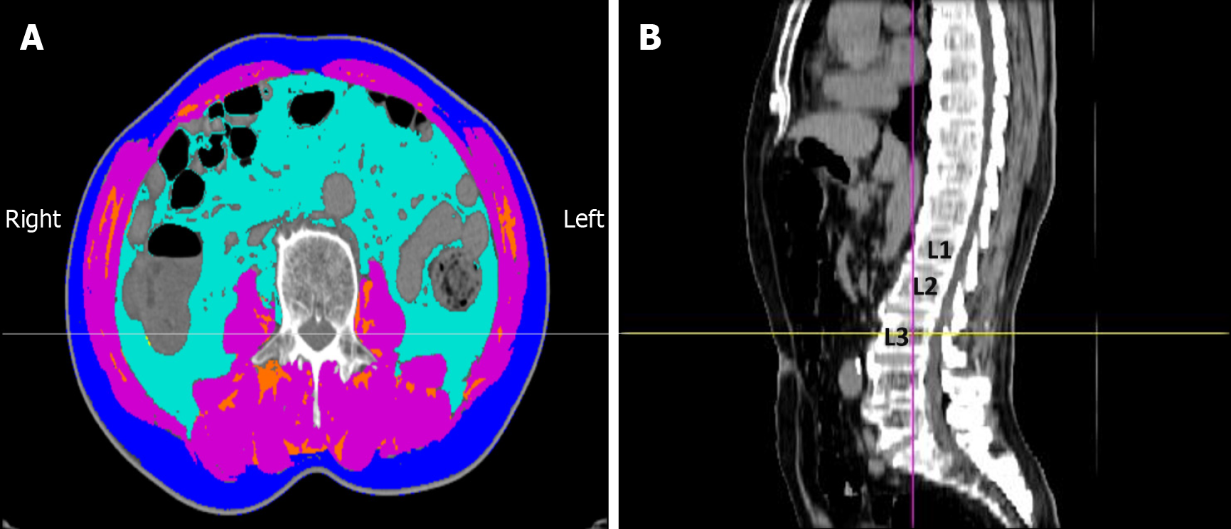
Figure 1 Assessment of body composition by computed tomography at the third lumbar vertebra (L3) level. A: Axial computed tomography (CT) image showing the segmentation of different tissue compartments: Skeletal muscle area (SMA) [pink, -29 to +150 Hounsfield units (HU)], visceral adipose tissue area (light blue, -150 to -50 HU), subcutaneous adipose tissue area (dark blue, -190 to -30 HU), and intermuscular adipose tissue area (orange, -190 to -30 HU); B: Sagittal CT image indicating the L3 level for axial analysis. The skeletal muscle index was calculated as the SMA divided by the square of the patient’s height (SMA/height²).

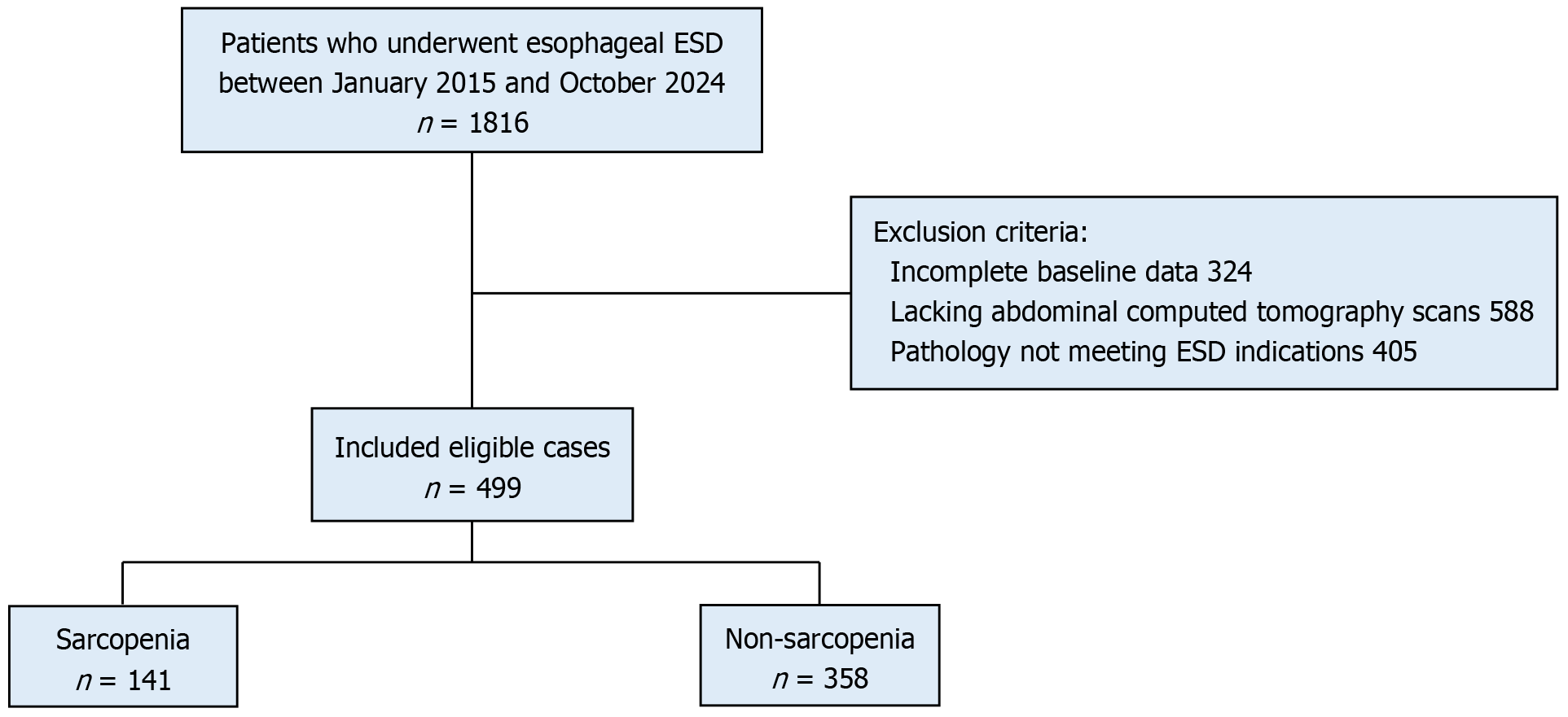
Figure 2 Flowchart of the study participants. ESD: Endoscopic submucosal dissection.

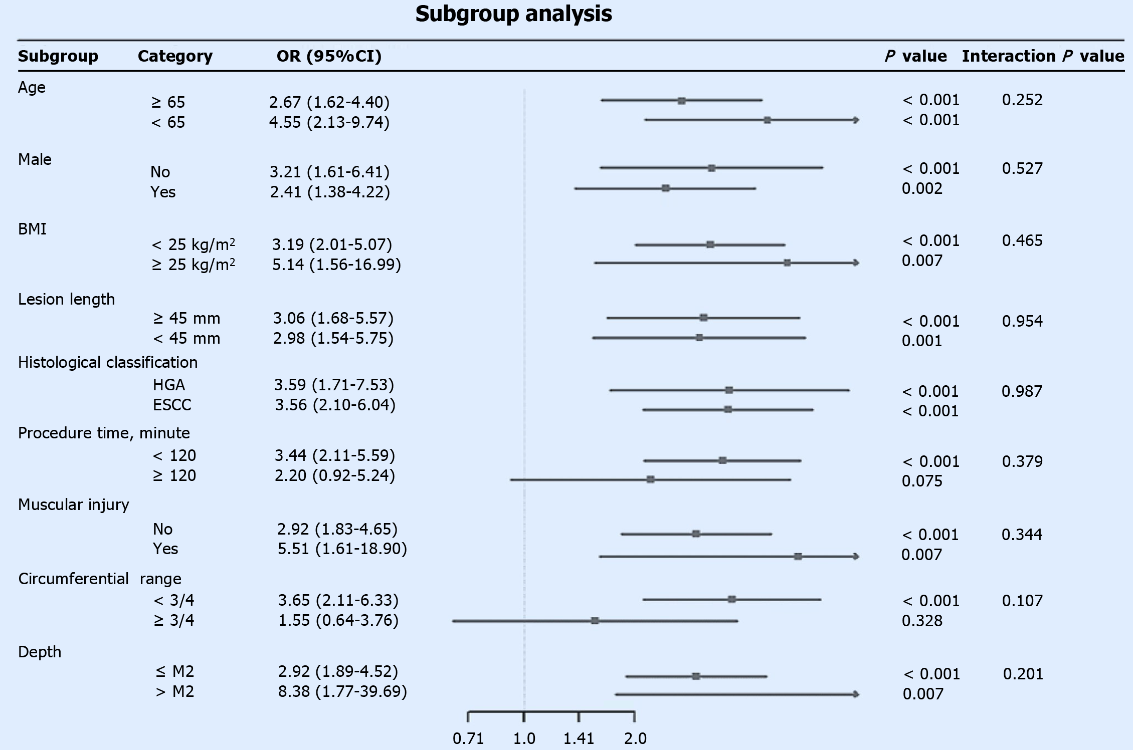
Figure 3 Subgroup analysis of the association between sarcopenia and postoperative stenosis risk. This forest plot displays the odds ratios (ORs) and 95% confidence intervals for the associations across various patient subgroups. An OR greater than 1 indicates a higher risk of stenosis in the sarcopenia group. The 'Interaction P' value tests whether the effect of sarcopenia on stenosis risk differs significantly between the subgroups. Circumferential: Circumferential resection range; ≤ M2: Invasion depth limited to the lamina propria mucosae or shallower; > M2: Invasion depth beyond the lamina propria mucosae. OR: Odds ratio; BMI: Body mass index; HGA: High-grade adenoma; ESCC: Esophageal squamous cell carcinoma.

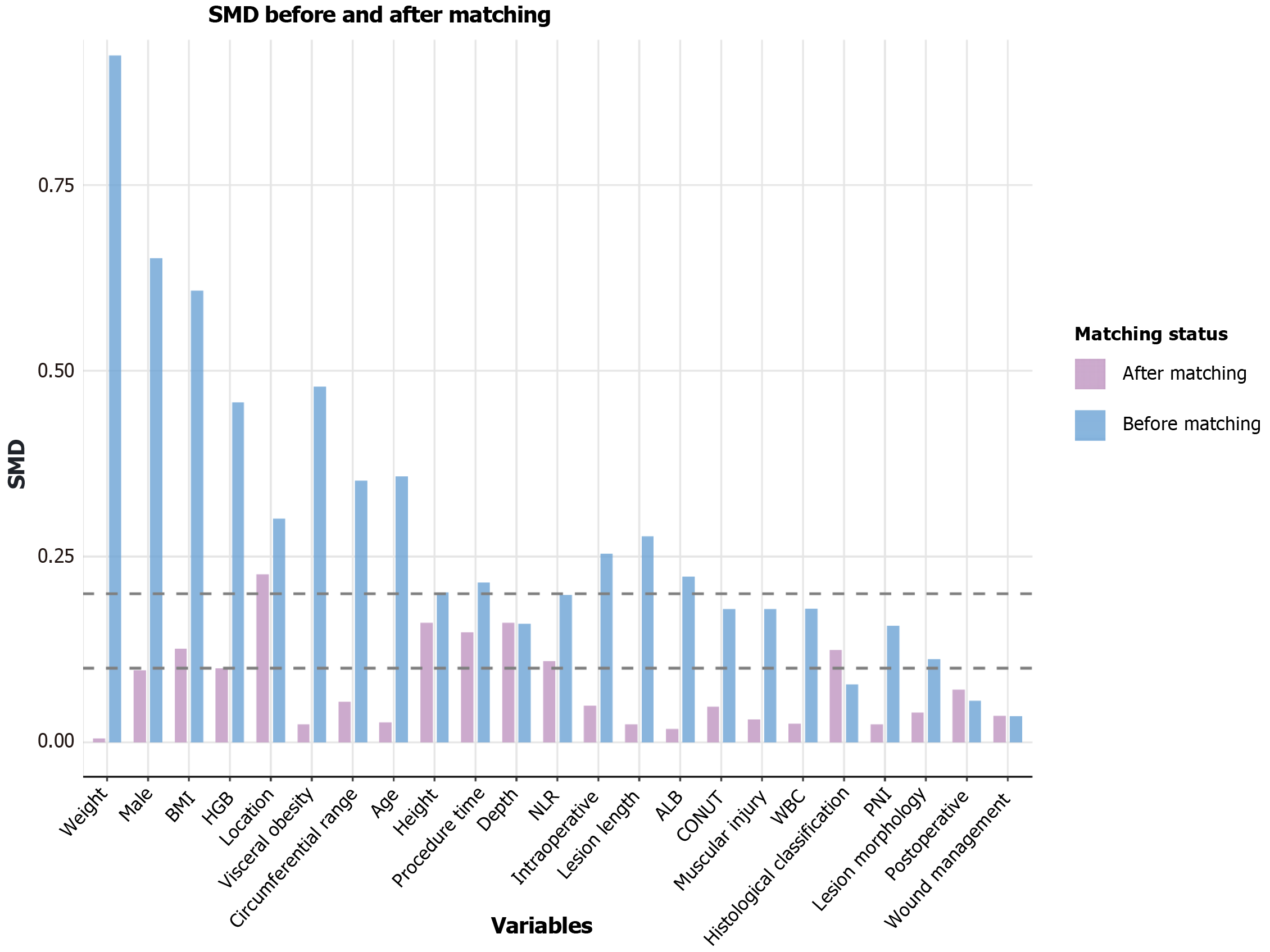
Figure 4 Assessment of covariate balance via standardized mean differences. The plot compares the standardized mean differences (SMDs) of the baseline variables before and after propensity score matching (caliper = 0.2). The results demonstrate that matching effectively improved the balance between the patient groups, as most post-matching SMDs fell below the 01 threshold. SMD: Standardized mean difference; BMI: Body mass index; CONUT: Controlling Nutritional Status score; PNI: Prognostic Nutritional Index; NLR: Neutrophil-to-lymphocyte ratio; WBC: White blood cell count; HGB: Hemoglobin concentration; ALB: Serum albumin concentration.

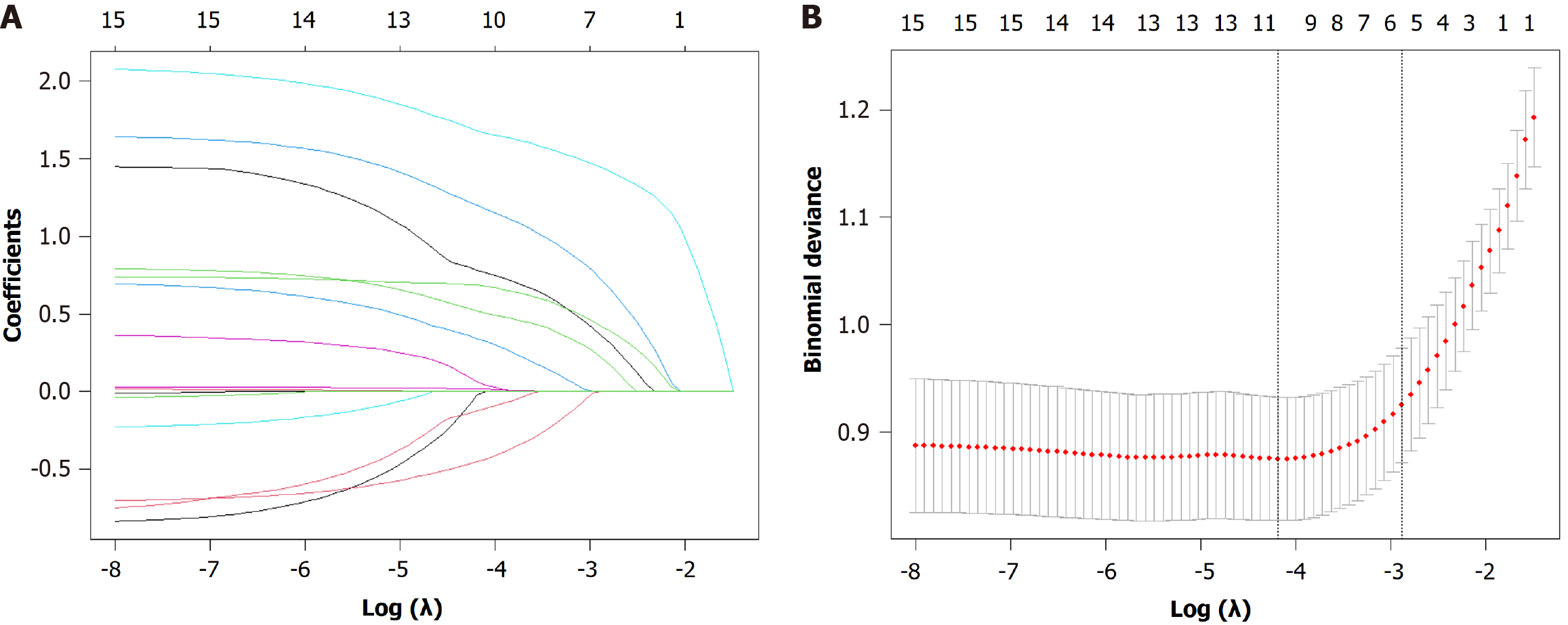
Figure 5 Variable selection using the least absolute shrinkage and selection operator regression model. A: The least absolute shrinkage and selection operator coefficient profile plot shows the trajectory of each variable's coefficient as the penalty parameter (lambda) increases. Each colored line represents a variable; B: The 10-fold cross-validation plot for tuning parameter (lambda) selection. The left vertical dashed line indicates the lambda value at which the model achieves minimum binomial deviance (λ.min), whereas the right dashed line represents the most regularized model within one standard error of the minimum (λ.1 se). The final predictors were selected at the λ.1 se value to obtain a more parsimonious model.

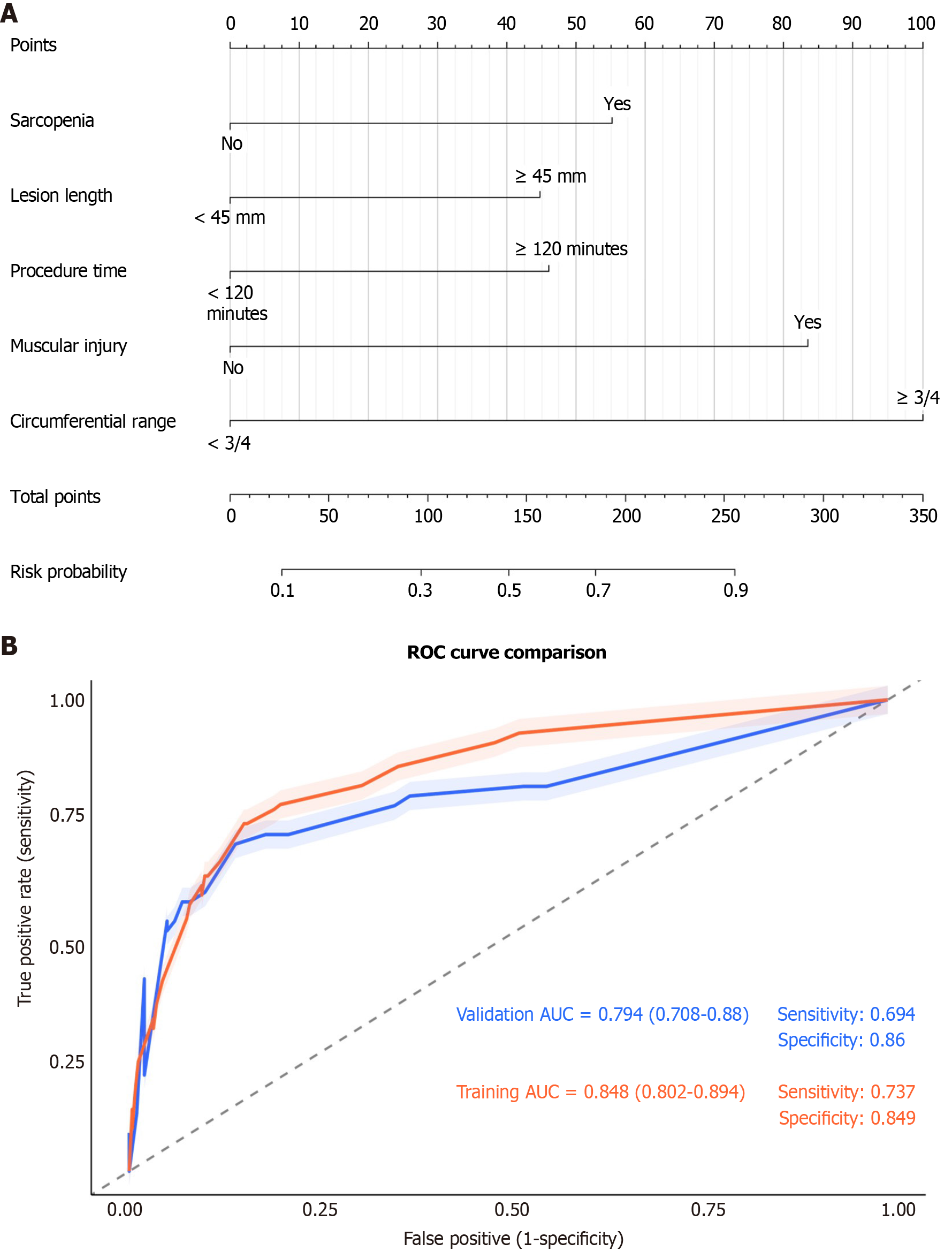
Figure 6 Development and validation of a predictive nomogram for post-endoscopic submucosal dissection stenosis. A: The nomogram is used to calculate an individual patient's risk of postoperative stenosis. For each predictor (including sarcopenia, lesion length, procedure time, and circumferential range), a vertical line is drawn upward to the 'Points' axis to determine the corresponding score. The sum of these scores is located on the 'Total Points' axis, and a line drawn downward to the 'Risk Probability' axis indicates the personalized stenosis risk; B: Receiver operating characteristic curves demonstrate the discriminative ability of the model. The area under the curve was 0.848 (95% confidence interval: 0.802-0.894) in the training cohort and 0.794 (95% confidence interval: 0.708-0.88) in the validation cohort, indicating good and consistent predictive performance. ROC: Receiver operating characteristic; AUC: Area under the curve.

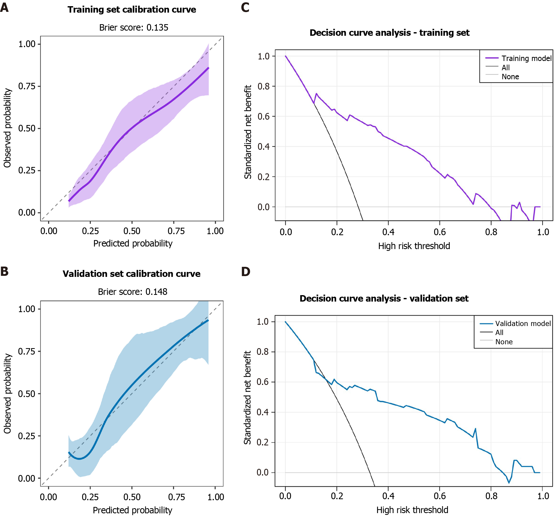
Figure 7 Calibration and decision curve analysis of the post-endoscopic submucosal dissection stenosis prediction model. A and B: Calibration curves plot the predicted probability against the observed frequency of stenosis. The dashed diagonal line represents perfect calibration. The close fit of the solid line (our model) to the diagonal, along with low Brier scores (training: 0.135; validation: 0.148), indicates excellent agreement between predictions and actual outcomes; C and D: Decision curve analysis evaluates the clinical net benefit of the model across various threshold probabilities. The “prediction model” line shows that using the nomogram for clinical decision-making provides greater net benefit than the strategies of “treating all” or “treating none” of the patients across a wide range of risk thresholds do, demonstrating its potential clinical utility.