Predicting lymph node metastasis in colorectal cancer using case-level multiple instance learning

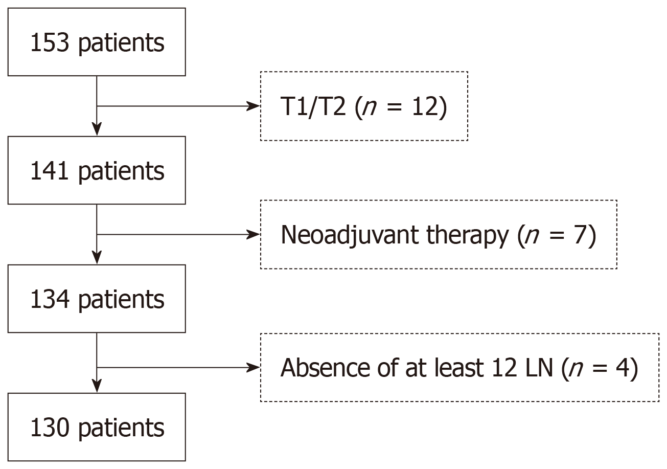
Figure 1 Diagram of inclusion/exclusion criteria for colorectal cancer data cohorts. LN: Lymph nodes.

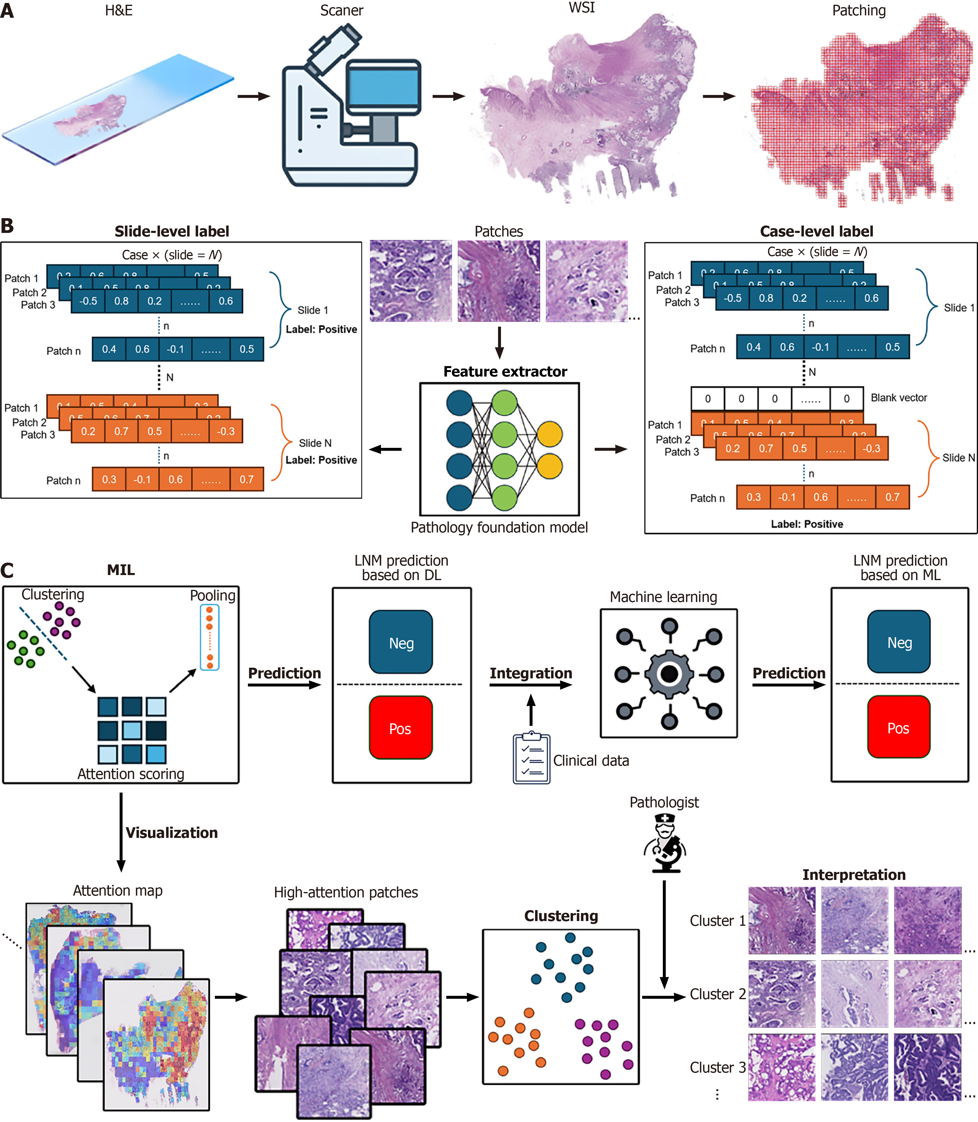
Figure 2 Workflow of case-level multiple instance learning for lymph node metastasis prediction in colorectal cancer histopathology. A: Data acquisition and preprocessing. Hematoxylin and eosin (H&E) stained slides from primary tumor resections are scanned using a digital scanner to generate whole-slide images (WSIs). WSIs are then processed into smaller, non-overlapping patches for subsequent analysis; B: Feature extraction with slide-level and case-level labeling. Slide-level label: For each slide, patches are extracted and fed into the feature extractor. Case-level label: Patches from all slides belonging to a single patient case are processed by the feature extractor; C: Multiple instance learning (MIL) Framework for lymph node metastasis (LNM) Prediction and Interpretation. MIL: Feature embeddings from patches of a case are input into the clustering-constrained-attention MIL framework. Attention scoring is applied to assign importance weights to different patches. Clustering is used to group similar patches. Pooling mechanisms aggregate these attention scores to generate a case-level or slide-level prediction. Attention scoring is applied to assign importance weights to different patches, potentially highlighting diagnostically relevant regions. Pooling mechanisms aggregate these attention scores to generate a case-level prediction. LNM prediction based on deep learning (DL): The MIL framework, utilizing deep learning, outputs a prediction for LNM (negative or positive). Integration: The DL based LNM prediction is integrated with clinical data to potentially enhance prediction accuracy. Machine learning: Integrated clinical and pathology features can be further analyzed using traditional machine learning classifiers to generate a final LNM prediction. H&E: Hematoxylin and eosin; WSIs: Whole-slide images; MIL: Multiple instance learning; LNM: Lymph node metastasis; ML: Machine learning; DL: Deep learning.

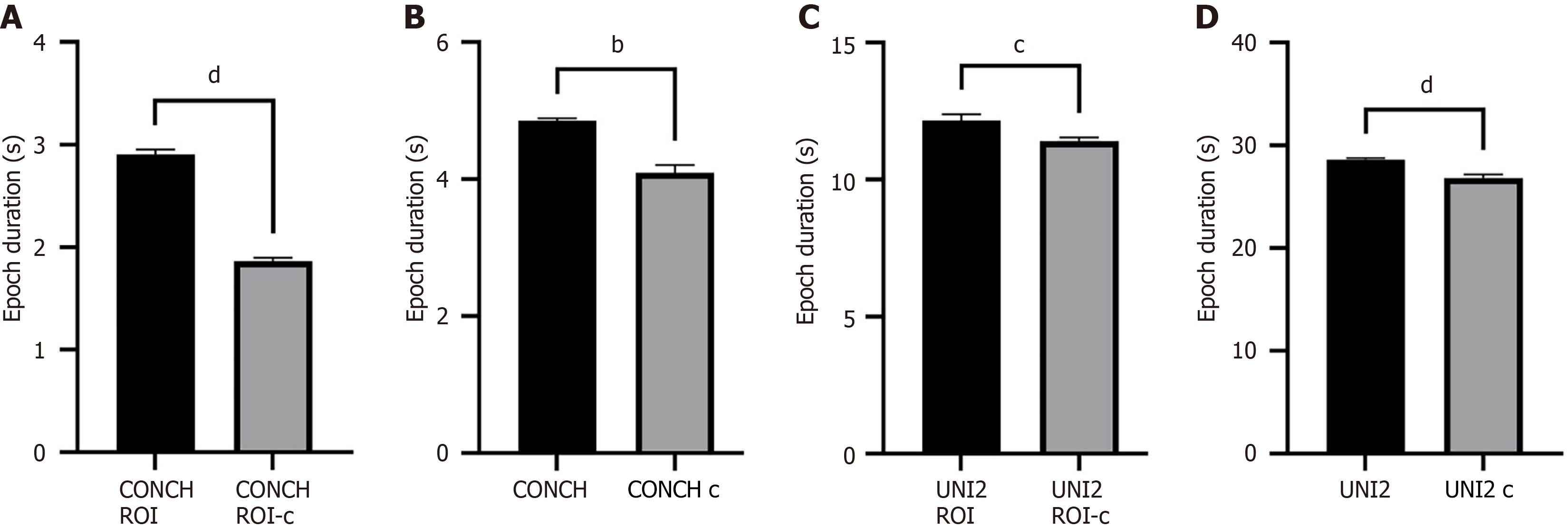
Figure 3 Comparison of computational efficiency across different model configurations. A: CONCH v1.5 model with pathologist-annotated regions of interest (ROI); B: CONCH v1.5 model without ROI annotations; C: UNI2-h model with ROI annotations; D: UNI2-h model without ROI annotations. Each panel displays the mean epoch duration (in seconds), comparing slide-level (black bars) and case-level (gray bars) training strategies. Data are presented as mean ± SD. Statistical significance was determined using a two-tailed unpaired t-test (A, C, D) or a Mann-Whitney U test (B). ^bP < 0.01, ^cP < 0.001, ^dP < 0.0001. ROI: Regions of interest.

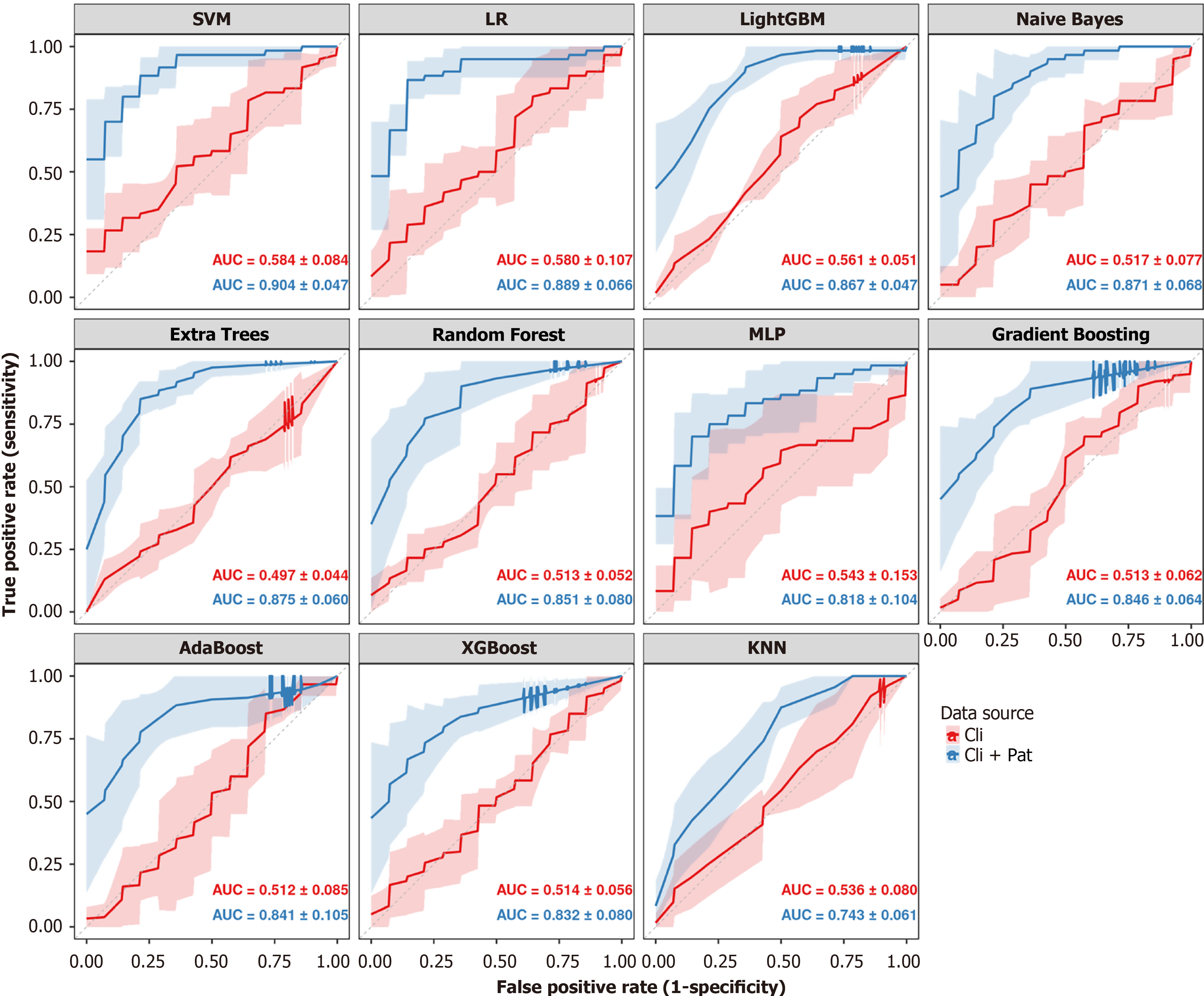
Figure 4 Comparative performance of machine learning models for predicting lymph node metastasis. This figure presents eleven panels, each dedicated to a different machine learning classifier. Within each panel, two receiver operating characteristic (ROC) curves are displayed to compare predictive performance based on different feature sets. The red curve represents the model trained using only clinical features ('Cli'), while the blue curve represents the model trained on combined clinical and deep learning-derived pathology features ('Cli + Pat'). The solid lines depict the mean ROC curve averaged across a 5-fold cross-validation, with the shaded areas representing the standard deviation. The corresponding mean area under the curve ± SD values for each feature set are annotated within each panel. SVM: Support vector machine; LR: Logistic regression; AUC: Area under the curve; KNN: K-nearest neighbours; GBM: Gradient boosting machine; MLP: Multilayer perceptron.

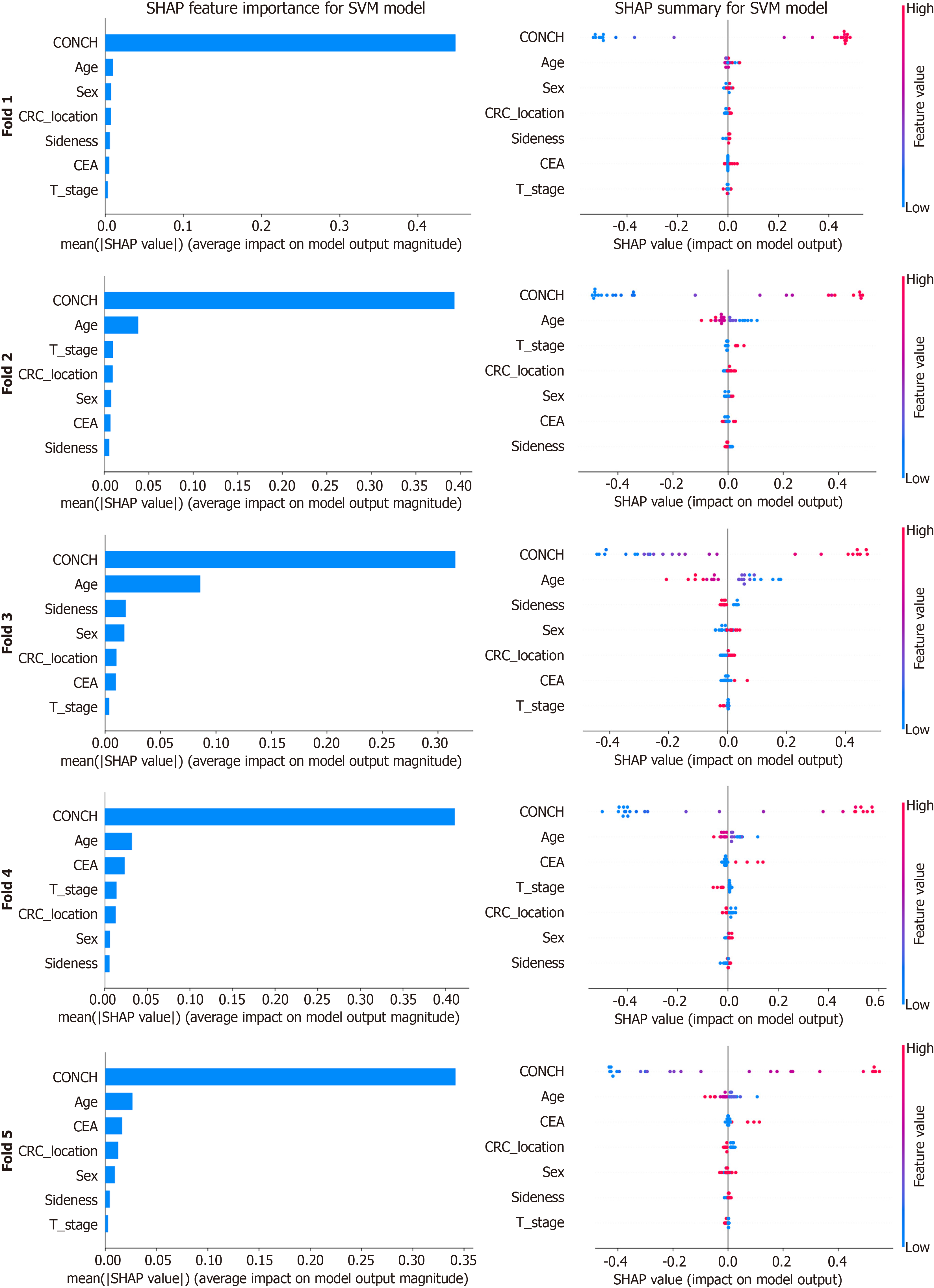
Figure 5 SHapley Additive exPlanations analysis of the top-performing support vector machine model. This figure presents a SHapley Additive exPlanations (SHAP) analysis of the top-performing support vector machine model across the five cross-validation folds. For each fold, overall feature importance is ranked by mean absolute SHAP value (bar charts, left), while corresponding summary plots (right) visualize the distribution and directional impact of SHAP values for individual predictions. In these plots, color indicates the original feature value (high in red, low in blue), revealing how feature levels drive model output. SHAP: SHapley Additive exPlanations; SVM: Support vector machine; CEA: Carcinoembryonic antigen; CRC: Colorectal cancer.

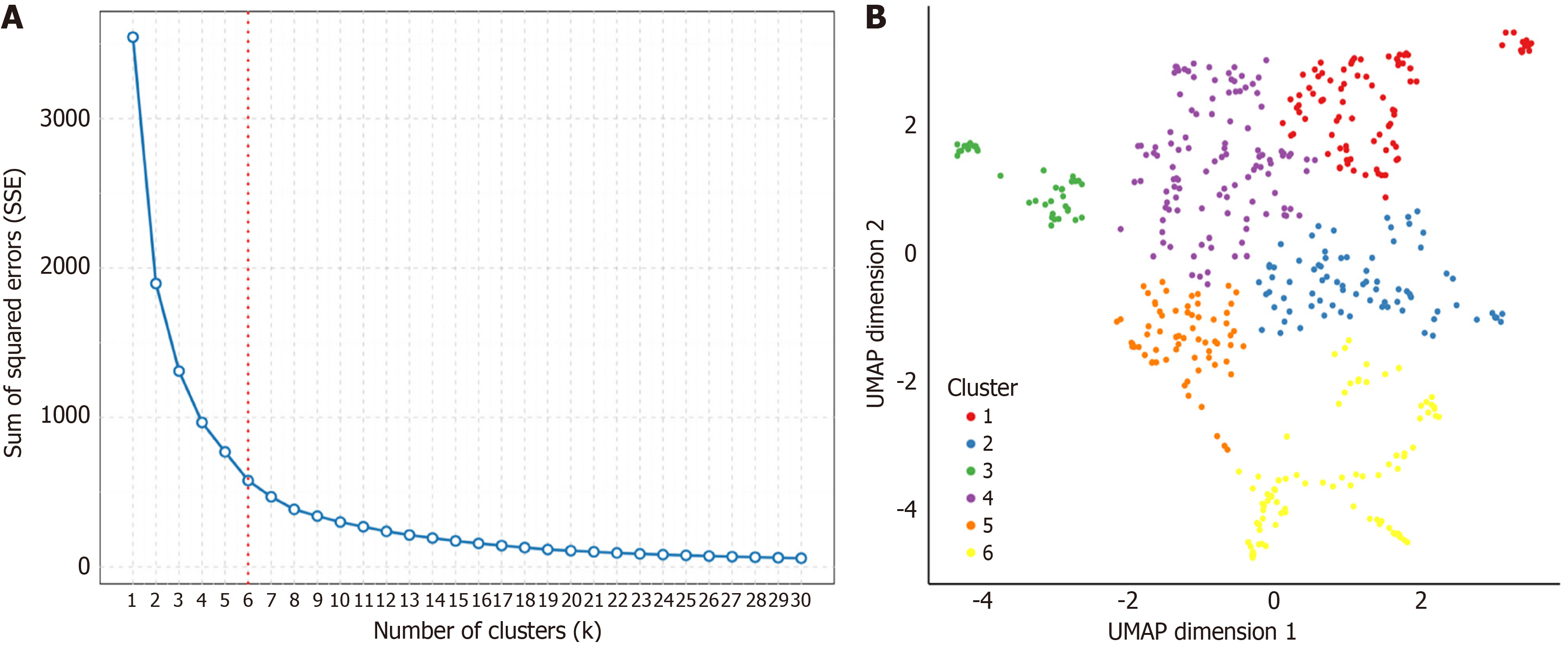
Figure 6 Clustering of high-attention histopathological features to identify morphological patterns. A: Elbow plot for determining the optimal number of clusters. The sum of squared errors is plotted against the number of clusters (k). The inflection point ("elbow") and the indicator line at k = 6 suggest that six is the optimal number of clusters for this analysis; B: Uniform Manifold Approximation and Projection visualization of high-attention tile embeddings, demonstrating separation into six distinct clusters. Each point represents an individual image tile, and its color denotes assignment to one of the six clusters as defined in the legend. SSE: Sum of Squared Errors; UMAP: Uniform Manifold Approximation and Projection.

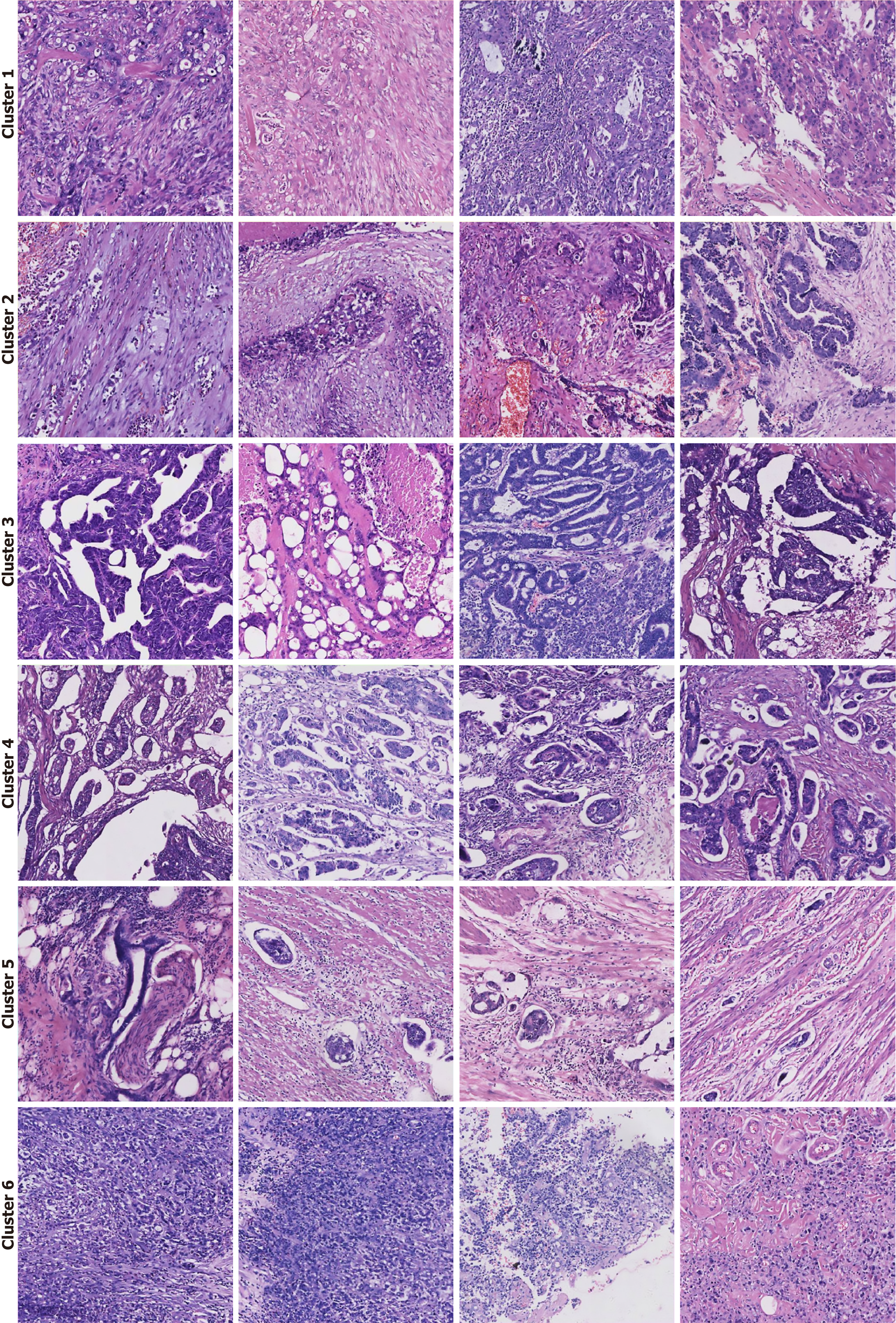
Figure 7 Histopathological interpretation of high-attention morphological clusters. Representative image tiles from the six distinct clusters identified by the deep learning model. Each cluster corresponds to a specific histopathological phenotype associated with lymph node metastasis risk. Cluster 1: Poorly differentiated adenocarcinoma, characterized by solid sheets and trabecular growth patterns with a high nuclear-to-cytoplasmic ratio. Cluster 2: Prominent desmoplastic reaction, showing a dense fibroblastic stromal response to invading tumor cells. Cluster 3: Adenocarcinoma with complex glandular architecture, featuring cribriform, fused, or back-to-back glands indicative of high-grade tumor organization. Cluster 4: Micropapillary adenocarcinoma, a high-risk pattern defined by small, cohesive tufts of tumor cells floating in stromal spaces without a true fibrovascular core. Cluster 5: Overt invasion, showcasing clear evidence of lymphovascular invasion and perineural invasion, where tumor cells infiltrate lymphatic channels and surround nerve fibers. Cluster 6: Signet-ring cell carcinoma, a distinct subtype composed of tumor cells containing large intracytoplasmic mucin vacuoles that displace the nucleus to the periphery.