
















Published online Oct 19, 2026. doi: 10.5498/wjp.123156
Revised: July 23, 2026
Accepted: September 4, 2026
Published online: October 19, 2026
Processing time: 154 Days and 1.8 Hours
Electroencephalography (EEG) topographic maps preserve the spatial arrange
To evaluate whether alpha-, beta-, and theta-band topographic maps provide different classification profiles under a controlled FusedNeXt framework.
A lightweight FusedNeXt architecture was evaluated using band-specific topographic maps generated from a retrospective, de-identified hospital EEG dataset. Each 15-second EEG segment was divided into five non-over
Under the fixed segment-level split, theta achieved the numerically highest window-level accuracy (85.24%), balanced accuracy (84.93%), macro F1-score (84.49%), and area under the curve (AUC) (0.9297); beta achieved 84.58% accuracy and an AUC of 0.9296, and alpha achieved 81.24% accuracy and an AUC of 0.8958. Under participant-grouped five-fold cross-validation, participant-level accuracy was 79.10% for theta, 77.84% for beta, and 74.66% for alpha. Beta and theta significantly outperformed alpha for balanced accuracy, macro F1-score, and AUC after Holm correction, whereas theta and beta did not differ significantly. Same-dataset baseline and ablation analyses provided additional evidence on model performance and component contribution. FusedNeXt contained approximately 7.17 million trainable parameters, required approximately 1.95 GFLOPs per forward pass, and classified one image in approximately 3 milliseconds.
The participant-grouped analysis provides an internal estimate of generalization to unseen participants within the same source dataset. The findings support band-specific discrimination within this cohort but do not establish diagnostic utility, a validated EEG biomarker, or external clinical validity. Independent external validation and more complete clinical phenotyping remain necessary.
Core Tip: This study presents a lightweight FusedNeXt-based framework for anxiety detection using electroencephalography (EEG) topographic map images. Instead of relying on handcrafted numerical features, alpha, beta, and theta frequency bands were converted into spatial scalp maps and evaluated under the same architecture, data split, and test protocol. The theta band achieved the best overall performance, while the beta band reduced false anxiety predictions in control samples. The proposed model provides competitive accuracy with low computational cost, supporting its potential use in fast EEG-based decision-support systems.
- Citation: Kaya S, Tasci G, Tuncer İ, Tasci B, Baygın N, Tasci I, Baygin M, Dogan S, Tuncer T. FusedNeXt-based anxiety detection from electroencephalography topographic maps: A comparative analysis of alpha, beta, and theta bands. World J Psychiatry 2026; 16(10): 123156
- URL: https://www.wjgnet.com/2220-3206/full/v16/i10/123156.htm
- DOI: https://dx.doi.org/10.5498/wjp.123156
Anxiety can affect cognitive, emotional, and physiological functioning[1,2] and can influence attention, perception, decision-making, sleep, and daily activity[3,4]. Clinical assessment relies primarily on interviews, rating scales, and self-report instruments[5,6]. These approaches remain essential, but physiological measurements may provide complementary information for computational mental-state analysis[7,8].
Electroencephalography (EEG) is a non-invasive method for recording brain electrical activity with high temporal resolution[9]. Anxiety-related changes have been investigated in EEG signals, and EEG-based methods have been applied to emotion recognition, mental-state classification, cognitive-load analysis, and neurological classification tasks[10,11]. However, EEG is nonlinear, non-stationary, noise-sensitive, and strongly variable across participants[12]. These characteristics make classification of anxiety-labelled clinical groups a challenging computational problem[13].
In EEG-based classification studies, handcrafted features based on time domain, frequency domain, time-frequency domain, and nonlinear analyses are widely used[14]. Although these features provide useful information about signal characteristics, they often require expert knowledge for feature design. In addition, these approaches can represent spatial relationships between EEG channels only to a limited extent[15]. In recent years, deep learning methods have been widely used in EEG-based classification problems due to their ability to automatically learn representations from data[16]. Convolutional neural networks (CNNs), recurrent networks, hybrid models, and attention-based approaches have been applied to different EEG classification problems. However, how EEG signals should be represented for the model remains a critical issue[17].
Direct use of raw EEG signals is advantageous in terms of preserving temporal patterns, but it may not always explicitly represent the spatial distribution of brain activity[18]. Feature vector-based approaches may largely lose the topographic structure depending on channel locations. In this context, EEG topographic map representation offers an effective alternative for transforming multi-channel EEG activity into a two-dimensional (2D) spatial image format[19]. In this representation, activity values obtained from EEG channels are projected onto a 2D plane according to the positions of electrodes on the scalp. Thus, the regional distribution of brain activity can be evaluated within an image-based structure.
Topographic map representation provides a particularly suitable data structure for convolutional deep learning models. Local intensity changes, regional activation patterns, and spatial relationships between channels can be directly learned from images. In this respect, the EEG topographic map approach establishes a meaningful bridge between neurophysiological signal analysis and image-based deep learning[20]. Especially in the classification of mental states, not only individual channel values but also the spatial distribution structure between different brain regions can carry discriminative information[21]. Frequency band analysis is another important component in EEG-based mental state evaluation[22]. Different EEG frequency bands may be linked to different neurophysiological processes[23]. For this reason, frequency-specific patterns should be examined. This may provide more detailed information than broadband EEG signals alone. In EEG-based anxiety studies, alpha, beta, and theta bands are important[24]. These bands are related to relaxation, arousal, attention, emotional regulation, and cognitive control[25]. However, their discriminative contribution may change across datasets, task structures, representation methods, and model types.
High classification performance alone is not sufficient for interpreting EEG-based anxiety-related group classification. The frequency representation, class-specific error distribution, validation unit, and balanced performance measures should also be examined[26-28]. These analyses help distinguish descriptive band differences from statistically supported and clinically meaningful conclusions.
Frequency-band-specific topographic representations therefore remain relevant to EEG-based anxiety classification research[29,30]. Comparing alpha, beta, and theta bands under the same experimental conditions can clarify whether their spatial representations produce different classification profiles[31]. The present study is positioned as a controlled band-comparison and model-evaluation study rather than as validation of a stand-alone clinical diagnostic test.
A review of EEG-based anxiety, emotional state, and mental state classification studies shows that different data representations and learning approaches have been used in the literature[13]. In these studies, various representation forms such as raw EEG signals, frequency band-based features, time-frequency representations, statistical measures, connectivity-based features, and topographic map images have been used[32]. In the classification stage, a wide range of methods has been preferred, from traditional machine learning methods to deep learning architectures[33]. Especially in recent years, CNN-based models, hybrid deep learning structures, and image-based EEG representations have attracted attention due to their automatic feature learning capacities[30].
In this context, recent studies on EEG-based mental state and anxiety detection were evaluated in terms of the dataset used, EEG representation form, method, validation strategy, and obtained results. A summary of the literature review related to the topic is given in Table 1[10,27,28,34-44]. Recent reviews have emphasized the methodological heterogeneity of artificial intelligence-based anxiety assessment. Ghonchi et al[45] reviewed anxiety-detection approaches based on neural and physiological signals and discussed the growing use of machine-learning and deep-learning models. Leccisotti et al[46] examined machine-learning-assisted resting-state EEG analysis across psychiatric disorders. Their review emphasized the diversity of diagnostic targets, EEG representations, feature sets, and classification methods. Liu et al[47] discussed major methodological challenges in physiological-signal-based stress and anxiety assessment. These challenges included small cohorts, demographic variability, signal-quality differences, incomplete reporting, model interpretability, data leakage, and limited external validation.
| Ref. | Task and cohort | EEG setting and representation | Model | Validation strategy | Best reported result | Relevance and main limitation |
| Baghdadi et al[34], 2019 | Two-level and four-level anxious-state classification; DASPS dataset with 23 participants | EEG was recorded with an Emotiv EPOC system during anxiety-inducing psychological stimulation. Handcrafted time-, frequency-, and nonlinear-domain features were used | Stacked sparse autoencoder and conventional classifiers | The participant-level validation protocol was not clearly reported | 83.50% accuracy for two levels and 74.60% for four levels | The study introduced the DASPS dataset and evaluated several EEG features. However, the cohort was small, and spatial topographic-map learning was not used |
| Chen et al[10], 2021 | Anxious-state classification in a closed neurofeedback setting | Frontal frequency-domain EEG features were extracted in an affective BCI-based neurofeedback paradigm | RBF-SVM with a one-vs-one strategy | The participant-level validation procedure was not clearly described | 92% accuracy | The study addressed anxiety in a specific neurofeedback paradigm. It did not use band-specific topographic maps or deep spatial learning |
| Mokatren et al[35], 2021 | Binary SAD vs HC classification; 32 SAD and 32 HC participants | Approximately 4 minutes of resting-state EEG; 34 channels; 1024 Hz. Wavelet-packet energy and entropy from five frequency bands were mapped to a 15 × 15 image-like representation | CNN, RBF-SVM, and kNN | Stratified subject-independent eight-fold cross-validation; eight participants were used for testing in each fold | 92.19% accuracy with CNN and the 2D image representation | Electrode geometry was preserved in an image-like structure. However, the individual contribution of alpha, beta, and theta topographic maps was not assessed |
| Shikha et al[36], 2021 | Anxiety classification; DASPS dataset with 23 participants | Time-, frequency-, and time-frequency-domain EEG features were extracted and subjected to feature selection | Stacked sparse autoencoder and conventional machine-learning classifiers | The participant-level validation strategy was not clearly reported | 83.93% accuracy with the stacked sparse autoencoder | The study evaluated complementary handcrafted features but did not use topographic maps or end-to-end spatial feature learning |
| Al-Ezzi et al[37], 2021 | Four-class SAD severity assessment; severe, moderate, mild, and HC groups with 22 participants per group | Six-minute eyes-closed resting-state EEG; 32 channels; 2048 Hz, downsampled to 256 Hz. PDC-based effective-connectivity matrices were produced for five frequency ranges | CNN, LSTM, and CNN-LSTM | Ten-fold cross-validation was reported. An additional 60-subject training and 28-subject testing analysis was presented | 93% average accuracy, 95% sensitivity, and 85% specificity with CNN-LSTM | Clinical SAD severity was assessed through effective connectivity. However, no external cohort was used, and the reported validation procedures were not fully uniform |
| Li et al[38], 2022 | Recognition of four anxiety levels | Comprehensive EEG features were extracted. Beta-band activity and frontal regions were reported as important | SVM | Participant-level fold construction was not clearly described | 62.56% accuracy | The study examined multiple anxiety levels but relied on handcrafted EEG features rather than image-based spatial representations |
| Muhammad and Al-Ahmadi[39], 2022 | Two-level and four-level state-anxiety classification; DASPS dataset with 23 participants | Channel-based mean power, RASM, and asymmetry features were extracted, mainly from theta and beta bands | RF, DT, kNN, SVM, and MLP | Leave-one-participant-out evaluation; samples from the test participant were excluded from training | 94.90% accuracy for two levels and 92.74% for four levels with RF | A participant-separated protocol and band-related features were used. However, topographic-map representation and deep spatial learning were not evaluated |
| Al-Ezzi et al[40], 2022 | Four-class SAD severity classification; 22 severe, 22 moderate, 22 mild, and 22 HC participants | Fuzzy entropy features were extracted from delta, theta, alpha, and beta bands | NB and other machine-learning classifiers | The participant-level validation procedure was not clearly documented | 86.93% accuracy, 92.46% sensitivity, and 95.32% specificity | Nonlinear EEG complexity was evaluated across several bands. The approach did not preserve electrode topology or use image-based learning |
| Shen et al[27], 2022 | Binary GAD vs HC classification; 45 GAD and 36 HC participants | Ten-minute eyes-closed resting-state EEG; 16 channels; 250 Hz. Four-second segments with 50% overlap were represented by PSD, fuzzy entropy, and PLI connectivity features | SVM, RF, and BP-bagging | Ten repetitions of an 80/20 hold-out split. Participant grouping was not clearly reported | 97.83 ± 0.40% accuracy and 97.95% F1-score with SVM | Spectral, nonlinear, and connectivity features were combined. Overlapping segments and unclear participant-level separation restrict direct comparison |
| Al-Ezzi et al[41], 2023 | Four-class SAD severity assessment; 66 SAD and 22 HC participants | Four-to-six-minute eyes-closed resting-state EEG; 32 channels; 2048 Hz, downsampled to 256 Hz. PDC and graph-theory features were extracted from four bands | SVM, kNN, LDA, NB, and DT | Explicitly reported subject-dependent ten-fold cross-validation | 92.78% accuracy, 95.25% sensitivity, and 94.12% specificity with SVM | Directed connectivity and network topology were assessed. Subject-dependent validation limits evidence for unseen-participant generalization |
| Liu et al[42], 2023 | Binary GAD vs HC classification; 45 GAD and 36 HC participants | Ten-minute resting-state EEG. High-frequency representations covering 4-30 Hz and 10-30 Hz were evaluated | MSTCNN with squeeze-and-excitation attention | The participant-level validation protocol was not clearly reported | 99.48% accuracy for 4-30 Hz and 99.47% for 10-30 Hz | Very high performance was reported for broad high-frequency EEG intervals. Controlled, separate alpha-, beta-, and theta-map comparisons were not performed |
| Ghonchi et al[43], 2024 | Binary normal vs anxious classification and four-class normal, light, moderate, and severe classification; DASPS dataset with 23 participants | Six anxiety-induction trials per participant; 14 electrodes. Beta-band EEG was transformed into sequences of 11 × 11 scalp maps | 2D CNN, squeeze-and-excitation attention, and LSTM | Five-fold cross-validation; participant-wise fold construction was not reported | 94.24% ± 0.33% accuracy for two classes and 92.58% ± 0.52% for four classes | This study is closely related because spatiotemporal scalp maps were used. However, only the beta band was evaluated, and participant-independent validation was not documented |
| Luo et al[28], 2024 | Four-level GAD grading; 39 controls, 9 mild, 38 moderate, and 33 severe GAD participants | Ten-minute eyes-closed resting-state EEG; 16 channels; 250 Hz. PLI connectivity features were extracted from theta, alpha1, alpha2, and beta bands | LightGBM, XGBoost, and CatBoost | Three repetitions of five-fold cross-validation with CCR resampling. Participant-wise fold construction was not reported | 98.1% ± 0.6% accuracy with CatBoost | A clinically relevant severity task was addressed. However, resampling was used, the validation unit was unclear, and the representation was connectivity-based rather than topographic |
| Adochiei et al[44], 2026 | HAM-A-based non-anxious, moderate, and severe categories; 16 in-house participants and 23 DASPS participants | Data from two EEG systems were harmonized to eight common channels. Spectral power, entropy, Hjorth, and DWT features were extracted | Logistic regression, MLP, and kNN | Nested cross-validation; five-fold inner model selection. Preprocessing, feature selection, PCA, scaling, and SMOTE were restricted to training folds | 87.5% accuracy and 0.859 F1-score with MLP; no severe case was correctly identified | A portable-EEG setting and a structured validation pipeline were used. However, the sample was small, two data sources were combined, and severe anxiety was substantially underrepresented |
Similar methodological diversity can be observed in the experimental studies summarized in Table 1. Baghdadi et al[34], Shikha et al[36], Li et al[38], and Muhammad and Al-Ahmadi[39] mainly used handcrafted time-domain, frequency-domain, nonlinear, or asymmetry-based EEG features. Some studies[37,40,41] assessed social anxiety and its severity through effective-connectivity, fuzzy-entropy, and graph-theory representations. Shen et al[27] combined spectral, nonlinear, and functional-connectivity features for generalized anxiety disorder (GAD) detection. Liu et al[42] used a multi-scale temporal CNN to model broad high-frequency EEG activity. Luo et al[28] combined phase lag index-based functional connectivity with ensemble learning for four-level GAD grading.
A smaller group of studies preserved some form of spatial electrode organization. Mokatren et al[35] mapped band-based EEG features to an image-like sensor configuration. Ghonchi et al[43] used temporal sequences of beta-band scalp maps with a CNN-attention-long short-term memory (LSTM) model. However, these studies did not provide a controlled comparison of alpha-, beta-, and theta-specific topographic maps under the same architecture, data split, training configuration, and evaluation protocol. Adochiei et al[44] evaluated portable EEG through multi-domain features and a nested validation pipeline. However, their small and heterogeneous cohort provided insufficient representation of severe anxiety.
The numerical results reported in Table 1 vary substantially. However, these results were obtained from different clinical definitions, class structures, participant cohorts, EEG systems, segment-generation procedures, feature representations, and validation units. Some studies used subject-dependent evaluation, while participant-level fold construction was unclear in several others. Direct numerical comparison is therefore inappropriate. The objective of the present study is narrower and methodologically controlled. Alpha-, beta-, and theta-band topographic maps were evaluated with the same FusedNeXt architecture, the same fixed 15-second EEG-segment-level split, training configuration, and test protocol. This design reduces the influence of model, data-size, and protocol differences during the descriptive comparison of the three frequency bands. The fixed-split performance metrics were calculated at the window/image level and should not be interpreted as subject-independent performance. Generalization to unseen participants was evaluated separately using participant-grouped five-fold cross-validation with participant-level probability aggregation. This additional analysis provides an internal estimate of unseen-participant generalization within the same source dataset; independent external generalization has not yet been established.
Many studies have been reported on EEG-based anxiety detection. However, important research gaps remain in current approaches. The main gaps that form the starting point of this study are summarized below: (1) Studies comparing alpha, beta, and theta bands under the same architecture, same data split, and same evaluation protocol are limited; (2) EEG studies are mostly based on numerical features, connectivity measures, or time-frequency representations. The evaluation of frequency band-specific EEG topographic map images with deep learning has remained more limited; (3) In vector-based feature approaches, electrode positions and topographic relationships between channels often cannot be adequately preserved; (4) In many studies, performance evaluation is mainly performed based on accuracy. Metrics such as class-based error behavior, balanced accuracy, macro F1-score, sensitivity, specificity, and AUC are not always considered together; and (5) For computational EEG classification frameworks, inference time and computational cost are also relevant alongside predictive performance. However, these quantities are not consistently reported in the literature. These gaps support examining frequency-band-specific topographic-map representations under controlled experimental designs for anxiety-related EEG classification.
EEG-based classification of anxiety-related clinical groups is an active area of computational mental-state research. Existing studies often rely on handcrafted features, connectivity measures, or numerical frequency-domain representations[27,41]. Although these methods can extract informative signal characteristics, they may represent scalp-electrode geometry only indirectly. In anxiety-related EEG research, discriminative information may occur not only in single-channel activity but also in spatial distributions across electrode locations[29,30].
The main motivation of this study is to model frequency band-specific spatial activation patterns in EEG signals within an image-based representation structure. For this purpose, raw EEG signals were not directly classified. Instead, EEG topographic map images were generated separately from the alpha, beta, and theta bands. Thus, regional activation distributions emerging in each frequency band were converted into a 2D image format and made directly processable by the deep learning model. Unlike classical vector-based feature representations, this approach preserves channel locations, regional intensity changes, and spatial relationships between channels in a more holistic way[30].
In the proposed method, alpha, beta, and theta bands were treated as separate experimental branches. The same window structure, topographic-map generation protocol, data split, FusedNeXt architecture, and evaluation metrics were used for all three bands. This controlled design reduces confounding related to sample count, model structure, and training protocol. The observed differences can therefore be compared as band-associated patterns within the present experimental framework, while causal attribution exclusively to frequency content requires appropriate statistical interpretation.
The study was designed not only to classify the available anxiety and control labels but also to compare the ability of alpha-, beta-, and theta-band topographic representations to support that classification under controlled conditions. The method consists of four main stages: EEG segmentation, band-specific decomposition, conversion of channel-level activity into 2D topographic maps, and separate FusedNeXt classification for each frequency band.
The FusedNeXt architecture was used to learn both local and more abstract spatial patterns from EEG topographic map images. In the basic structure of the model, group convolutions, the Gaussian Error Linear Unit (GELU) activation function, batch normalization layers, and additive fusion connections were used together. This structure enables complementary features obtained from different convolutional transformation paths to be combined in a common representation space. Thus, the model can learn multi-component topographic patterns that can distinguish anxiety and control classes without depending on a single linear feature extraction flow.
Another objective was to avoid relying on overall accuracy alone. Therefore, performance was evaluated with balanced accuracy, macro precision, macro recall, macro specificity, macro F1-score, class-specific sensitivity and specificity, confusion matrices, and receiver operating characteristic (ROC)-area under the curve (AUC) in addition to accuracy. This broader evaluation is particularly relevant when sample counts are not fully balanced[26].
Overall, the study presents a controlled analysis framework that combines frequency-band-specific EEG topographic maps with FusedNeXt for classification of the available anxiety and control labels. Alpha, beta, and theta bands were compared under matched experimental conditions, and the framework was further evaluated through participant-grouped validation, same-dataset baselines, ablation analysis, and statistical testing.
Previous EEG-based anxiety studies have mainly used handcrafted spectral, nonlinear, asymmetry, and connectivity features. For example, Shen et al[27] combined spectral, entropy, and functional-connectivity measures, while Al-Ezzi et al’s studies[37,40,41] used effective-connectivity, fuzzy-entropy, and graph-theory representations. Luo et al[28] also used functional-connectivity features with ensemble learning. Although these approaches can represent frequency-specific EEG characteristics, conventional feature vectors do not inherently retain electrode geometry unless spatial coordinates or channel adjacency are explicitly encoded.
Preserving electrode positions is important because EEG activity is spatially distributed across the scalp. Anxiety-related information may be associated with regional intensity differences, hemispheric asymmetries, and relationships between neighboring or distant brain regions. When channels are represented only as an unordered feature vector, these spatial relationships may not be directly available to the learning model. Topographic maps retain the approximate spatial arrangement of the electrodes and convert regional EEG activity into an image-like representation. This allows convolutional models to learn local spatial patterns, regional gradients, and interregional differences from the scalp representation[19,30].
EEG spatial representations have previously been used for anxiety detection. Mokatren et al[35] mapped band-based EEG features to a 2D sensor configuration and reported improved classification performance with a CNN. However, the individual contributions of alpha, beta, and theta topographic representations were not evaluated under separate but identical experimental conditions. Ghonchi et al[43] transformed beta-band EEG signals into temporal sequences of scalp maps and used a CNN-attention-LSTM model. However, that study focused only on the beta band, and participant-independent fold construction was not clearly documented. Therefore, the use of EEG scalp maps itself is not claimed as the primary novelty of the present study.
The methodological contribution of the present work lies in the controlled comparison of alpha-, beta-, and theta-band topographic maps under matched experimental conditions and complementary validation protocols. The fixed 15-second EEG-segment-level split was retained for direct comparison of band-specific window-level results, while participant-grouped five-fold cross-validation was used to estimate generalization to unseen participants within the same source dataset. The same map-generation procedure, participant folds, FusedNeXt architecture, training configuration, and evaluation protocol were applied across bands. Same-dataset baseline, ablation, and statistical analyses were used to support architecture-related and band-related interpretations.
A further methodological difference is the use of the proposed FusedNeXt architecture for EEG topographic-map classification. Previous anxiety studies have used conventional CNNs, CNN-LSTM models, support vector machines, ensemble classifiers, and multi-scale temporal CNNs[27,28,35]. In contrast, FusedNeXt combines grouped convolutions, additive multi-path fusion, a patchify-style stem, and a transformer-inspired inverted-bottleneck channel-mixing block within a hierarchical fully convolutional structure. The architecture was designed to learn local and higher-level spatial patterns while maintaining a relatively compact computational structure. Experimental performance and computational results are reported only in the results and discussion sections.
This study was conducted as a retrospective secondary computational analysis of a previously collected and de-identified hospital EEG dataset. The participants were not recruited specifically for the present computational study. No prospective sample-size calculation or statistical power analysis was performed. All available stored EEG segments from the two selected clinical groups were included after data organization. Therefore, the study population represents a convenience clinical cohort rather than a prospectively powered research cohort.
The dataset included 88 participants: 44 labelled anxiety and 44 labelled control. Group labels were obtained from the available hospital clinical records and clinical assessment. Anxiety denotes the available hospital-derived clinical group label; it should not be interpreted as a uniformly phenotyped anxiety subtype or as a diagnosis reconstructed from a standardized research protocol. Control denotes the absence of an active psychiatric finding in the available assessment; it should not be interpreted as a fully characterized research-grade healthy-control cohort.
The de-identified dataset did not retain uniform individual DSM/ICD codes, the specific diagnostic-manual version used for individual participants, structured diagnostic interview records, validated anxiety-scale scores or cut-off values, detailed anxiety-subtype information, or complete demographic and clinical variables. Therefore, age, sex, education level, medication use, psychiatric and physical comorbidities, symptom severity, and subtype-specific group differences could not be systematically evaluated. No unverified clinical or demographic information was reconstructed.
The control group included participants with no active psychiatric finding recorded in the available clinical assessment. However, the available information was not sufficient to define these participants as a fully characterized research-grade healthy-control cohort. Complete demographic and clinical variables were not retained in structured form. Therefore, age, sex, education level, medication use, psychiatric comorbidity, physical comorbidity, and other possible group differences could not be evaluated.
EEG signals were sampled at 200 Hz. The available montage contained 22 channels: Fp1, Fp2, F3, F4, C3, C4, P3, P4, O1, O2, F7, F8, T3, T4, T5, T6, Fz, Cz, Pz, E, A1, and A2. The E, A1, and A2 channels were not treated as cortical electrode positions during topographic-map generation. Therefore, the topographic maps were generated from the remaining 19 cortical EEG channels.
The retrospective de-identified dataset contained stored 15-second EEG segments obtained from the original clinical EEG recordings. Each 15-second segment was divided into five non-overlapping 3-second windows. Each window contained 600 samples at the sampling frequency of 200 Hz. The exact EEG device model, acquisition reference, impedance threshold, hardware-filter settings, total duration of the original EEG recordings, and original recording condition were not retained in the de-identified dataset. Therefore, these acquisition parameters and whether the original recordings represented a standardized resting-state or task-related condition could not be retrospectively verified.
The available data consisted of stored 15-second EEG segments obtained from the clinical recordings. The term “segment” refers to one stored 15-second signal section. It does not refer to an experimental trial or behavioral task. No experimental task was applied as part of the present retrospective computational analysis. Each 15-second EEG segment was divided into five non-overlapping 3-second windows. Each window contained 600 samples at the sampling frequency of 200 Hz. Therefore, each 15-second EEG segment produced five topographic-map images per frequency band. The same segmentation procedure was applied to the alpha, beta, and theta bands.
The anxiety group contained 1712 stored 15-second EEG segments, whereas the control group contained 1041 segments. The difference in segment counts resulted from the unequal numbers of stored EEG segments available for the two clinical groups. For each frequency band, the complete dataset contained 13765 topographic-map images. The anxiety group contributed 8560 images, and the control group contributed 5205 images. The training partition contained 11015 images per band, whereas the test partition contained 2750 images per band. The same EEG segments, window indices, and partition assignments were used for the alpha, beta, and theta experiments. Therefore, all three band-specific experiments contained the same number of images and used the same internal data split. The distribution of participants, 15-second EEG segments, and generated topographic-map images across the training and test partitions is summarized in Table 2.
| Data split | Class | Unique participants represented in the partition | Number of 15-second EEG segments | Topographic-map images per band | Topographic-map images across the three bands |
| Train | Anxiety | 44 | 1370 | 6850 | 20550 |
| Train | Control | 43 | 833 | 4165 | 12495 |
| Test | Anxiety | 43 | 342 | 1710 | 5130 |
| Test | Control | 41 | 208 | 1040 | 3120 |
| Total | Anxiety | 44 | 1712 | 8560 | 25680 |
| Total | Control | 44 | 1041 | 5205 | 15615 |
| Total | All | 88 | 2753 | 13765 | 41295 |
An approximately 80:20 stratified hold-out split was initially applied at the 15-second EEG-segment level before each segment was divided into five non-overlapping 3-second windows. All five windows derived from the same segment were retained in the same partition. The training partition included segments from 44 unique anxiety participants and 43 unique control participants. The test partition included segments from 43 unique anxiety participants and 41 unique control participants. These participant counts are not additive because different segments from the same participant could occur in both partitions. Therefore, the results obtained from this fixed split were considered window-level internal estimates and were not interpreted as subject-independent performance.
The participant was the unit of clinical labeling, whereas each 3-second EEG window and its corresponding topographic map represented the model input unit. To evaluate generalization without participant overlap, an additional participant-grouped five-fold cross-validation analysis was performed. Participant identity was used as the grouping variable, and all segments and windows from the same participant were assigned to the same fold.
Participant identity was not used as a grouping variable during the split. Consequently, different EEG segments from the same participant could occur in both the training and test partitions. The participant counts reported for the two partitions are therefore not additive. This overlap may produce correlated samples across the partitions and may lead to optimistic performance estimates.
Accordingly, the reported accuracy, balanced accuracy, sensitivity, specificity, precision, F1-score, and AUC values represent window-level internal estimates obtained under the fixed segment-level split. These fixed-split results do not establish subject-independent generalization or participant-level diagnostic performance because participant overlap was present between the partitions. Generalization to unseen participants was therefore evaluated separately using participant-grouped five-fold cross-validation, as reported in robustness, baseline, and statistical validation section. However, this additional analysis remains an internal validation within the same source dataset and does not replace independent external validation.
Despite this limitation, the same internal split was used for the alpha, beta, and theta experiments. The same EEG segments, windows, FusedNeXt architecture, training configuration, and evaluation procedure were applied to all three bands. Therefore, the observed differences among the frequency-band results should be interpreted only as descriptive comparisons within the analyzed dataset.
Overall pipeline overview: In this study, a lightweight deep learning framework, named FusedNeXt, is proposed for classification of band-specific EEG topographic maps associated with the available anxiety and control labels. The architectural design of FusedNeXt is inspired by two complementary lines of work in modern deep learning. The first source of inspiration is the hyper-connection principle, in which feature maps generated by parallel transformation paths are fused through additive interactions rather than being processed along a single sequential pipeline. The second source of inspiration is the transformer family, particularly its inverted-bottleneck channel-mixing block (i.e., the position-wise feed-forward module), in which a low-dimensional representation is first projected into a higher-dimensional space through nonlinear activation and then projected back. FusedNeXt combines these two ideas inside a fully convolutional, group-convolution-based topology so that spatial mixing and channel mixing are realized through a hyper-connected, additively fused multi-path block. The architecture is designed to learn complementary local and higher-level topo
The full pipeline of the proposed framework consists of four sequential stages: (1) Windowing: Each stored 15-second EEG segment is divided into five non-overlapping 3-second windows. This procedure provides five model-input windows per segment while preserving the temporal locality of the original stored segment; (2) Band decomposition: Each window is decomposed into three frequency bands of interest: Alpha, beta, and theta. The same decomposition protocol is applied to all windows; (3) Topographic map generation: Band-specific channel activity values are projected onto a 2D scalp plane using the standard electrode coordinates, yielding a three-channel RGB topographic map image of size H × W × 3; and (4) FusedNeXt-based classification: The topographic image is fed to the proposed FusedNeXt network, which produces an anxiety/control class probability vector.
The alpha, beta, and theta bands were treated as separate experimental branches. The same 15-second EEG-segment-level partition assignments, windowing procedure, FusedNeXt architecture, training configuration, and evaluation protocol were used for all three bands in the fixed internal analysis. This design reduced the influence of differences in sample size, model structure, and evaluation procedure. The fixed-split results were interpreted as window-level internal estimates, while participant-grouped five-fold cross-validation was used separately to assess generalization to unseen participants. The overall pipeline is illustrated in Figure 1.

As shown in Figure 1, the proposed method addresses the stages of band-specific filtering, topographic mapping, deep feature learning, and classification in an integrated framework, starting from the stored 15-second EEG segments available in the retrospective dataset. This framework evaluates not only band-specific EEG activity but also its inter-channel spatial relationships within an image-based representation. Thus, channel-level band-power values are converted into 2D topographic images that can be processed directly by deep learning models.
In this study, the alpha, beta, and theta bands were treated as separate experimental arms. The same data split strategy was used for each band. The same model architecture and evaluation protocol were also applied. With this approach, the three band-specific representations were compared under matched data size, model architecture, and experimental settings. This controlled framework supports a focused analysis of differences associated with alpha, beta, and theta topographic maps. The interpretation of those differences is based on both the fixed internal results and the participant-grouped statistical analyses reported later in the manuscript.
EEG band decomposition and topographic map generation: Let a stored 15-second EEG segment be denoted by S∈ℝNc×T, where Nc is the number of channels and T is the number of temporal samples. The segment is first divided into five non-overlapping windows
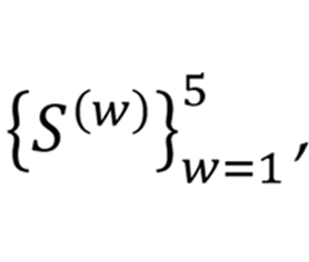
where S(w)∈ℝNc×Tw and
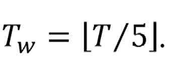
Each window was separately bandpass-filtered into the alpha, beta, and theta frequency bands using a zero-phase finite-impulse-response bandpass filtering procedure. The same filtering procedure was applied to all participants and windows within each frequency-band experiment. Let B∈{α, β, θ} denote the band of interest with a passband
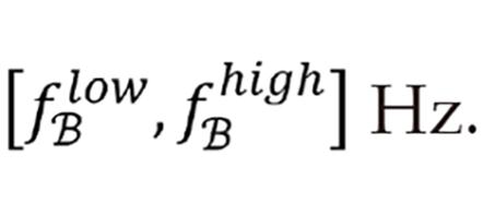
The band-specific signal is obtained by: S(w,B) = hB * S(w), B∈{α, β, θ} (1), where hB denotes a zero-phase finite-impulse-response bandpass filter for band B and * denotes convolution along the time axis. No independent component analysis (ICA), EOG regression, automated eye-movement artifact correction, automated muscle-artifact rejection, or bad-channel interpolation was applied as part of the preprocessing pipeline before band-power calculation. No missing-channel imputation was applied. Therefore, residual ocular and muscular activity may have remained in the analyzed EEG segments. This limitation was considered during the interpretation of the frequency-band-specific results.
Channel-wise band power is then computed as:
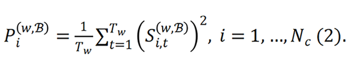
This produces a power vector p(w,B)∈ℝNc for each band of each window. After bandpass filtering, the band-specific power of each cortical EEG channel was calculated separately for each 3-second window as the mean squared amplitude of the filtered signal, as defined in equation (2). This procedure produced one channel-wise power vector for each window and frequency band. The resulting values represented direct band-specific mean-squared amplitudes; no relative-power normalization or logarithmic transformation was applied before spatial mapping. The 19 cortical EEG channels corresponded to standard scalp locations of the International 10-20 electrode system, and the channel-wise power values were mapped to these spatial locations. The discrete channel-wise power values were then interpolated onto a regular 2D scalp grid to obtain a continuous spatial representation. The resulting spatial power distribution was rendered as a three-channel topographic-map image. Each topographic map was generated at an input size of 224 × 224 × 3 and was subsequently provided to the FusedNeXt model.
The same electrode coordinates, spatial mapping procedure, image dimensions, and color-mapping procedure were used for the alpha, beta, and theta branches. Therefore, the topographic-map generation procedure was kept constant across the three frequency-band experiments. The exact interpolation kernel, interpolation-specific parameters, and the scope of color-scale normalization used in the archived map-generation procedure could not be retrospectively verified from the available analysis records. Therefore, these parameters are not reported to avoid introducing unverified methodological information. Although the same map-generation procedure was applied consistently to all experimental branches, the absence of these archived implementation details limits exact methodological reproducibility and is acknowledged as a limitation of the retrospective study.
The vector p(w,B) is then projected onto a 2D scalp plane using the standard electrode coordinates
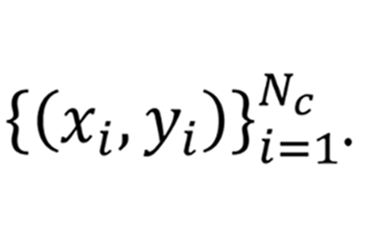
Let T(.) denote the topographic map operator, which combines: (1) Interpolation of channel-wise power values onto a regular 2D grid; and (2) Standard colormap rendering. The band-specific topographic map image is obtained by:

with H = W = 224. The same operator T(.), the same windowing, and the same colormap are used for all three bands. As a result, the only experimental factor that varies across bands is the frequency content of the underlying signal, which makes the band comparison strictly controlled. Alpha, beta, and theta were selected for the controlled single-band analysis because these frequency ranges have been frequently associated with anxiety-related arousal, attention, emotional regulation, and cognitive control. The same windowing, band-power calculation, topographic-map generation, model architecture, and evaluation protocol were applied to all three bands. Therefore, the primary experimental objective was to compare the spatial representations produced separately by these frequency components.
Delta and gamma bands were not included because the available preprocessing pipeline did not permit sufficiently reliable control of their principal confounding factors. Delta-band activity may be affected by slow baseline drift, electrode instability, and variations in vigilance or drowsiness. Gamma-band activity recorded from the scalp is particularly susceptible to contamination from facial and cranial muscle activity. Since ICA, EOG regression, and automated muscle-artifact rejection were not included in the preprocessing pipeline, the cortical origin of gamma-band differences could not be evaluated with sufficient confidence. Multi-band fusion was also outside the scope of the controlled single-band comparison. Such an analysis represents a separate research question and requires dedicated early-, feature-, or decision-level fusion experiments. Representative band-specific topographic map images are shown in Figure 2. The sample images in Figure 2 present frequency-band-specific EEG activity in the form of topographic maps. Different frequency bands can produce different activation distributions over the scalp.

In this study, the same topographic map generation protocol was used for all frequency bands. Thus, the comparison among the alpha, beta, and theta bands was based only on frequency content. The image generation method was kept constant across bands. The windowing strategy was also kept constant. The data organization was also kept constant. Only the EEG component related to the selected frequency band was changed. With this design, the comparative analysis structure of the study was strengthened. A more reliable band-based evaluation was also provided.
The proposed FusedNeXt network is a hierarchical, fully convolutional architecture designed around three principles: (1) Hyper-connected multi-path computation. Inside each block, the input feature map is processed by two or three parallel paths, and the resulting feature maps are merged by additive fusion - i.e., element-wise summation in a shared representation space. This is the convolutional analogue of hyper-connections: Instead of forwarding the signal through one path, we forward it through several complementary paths and then sum; (2) Transformer-style inverted-bottleneck channel mixing. Each block contains a transformer-style channel mixer in which a 1 × 1 grouped convolution expands the channel dimension by an expansion ratio r = 4, applies a GELU nonlinearity, and a 1 × 1 convolution projects it back. This is the convolutional version of the position-wise feed-forward block of a transformer encoder; and (3) Group-convolutional efficiency. All convolutions other than the projection are grouped. This drastically reduces parameter count and FLOPs and is the main mechanism that makes FusedNeXt lightweight. The network has four hierarchical stages with channel widths C1 = 96, C2 = 192, C3 = 384, C4 = 768, preceded by a stem block and connected by transition blocks. The overall topology is depicted in Figure 3.

As shown in Figure 3, the FusedNeXt model first converts the topographic map image into a low-dimensional but more feature-rich channel map. In subsequent stages, while the number of channels is increased, the spatial resolution is gradually reduced. This process enables the model to learn local color and intensity variations in the early layers, and more meaningful and abstract spatial patterns in terms of class discrimination in the deeper layers. The convolutional transitions used between stages contribute to the controlled transformation of the feature maps.
The deep feature maps obtained in the final layer of the architecture are converted into a compact vector representation using a global average pooling layer. Subsequently, a two-output classification head is used to generate probability values for the anxiety and control classes for each image. During the training process, the model’s learnable parameters were optimized end-to-end. As a result, the FusedNeXt architecture was trained to learn regional activation patterns directly from the EEG topographic-map inputs.
Let X∈ℝH×W×3 denote an input EEG topographic map image with H = W = 224. We denote by Convk×k(.) a standard 2D convolution with kernel size k×k, by
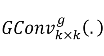
a grouped 2D convolution with g(.) groups, by BN(.) batch normalization, and by σ(.) the GELU activation. Bias terms are absorbed into the convolution operators for clarity.
Stem block: The stem block performs initial feature embedding and spatial downsampling. It applies a 4 × 4 convolution with stride 4, followed by batch normalization and GELU activation:

with C1 = 96. The stem reduces spatial dimensions from 224 × 224 to 56 × 56 and lifts the representation from 3 channels to 96 channels in a single operation. This patchify-style stem is itself inspired by the vision-transformer patch embedding and provides a strong, low-cost initial token-like feature.
FusedNeXt block: Each FusedNeXt stage s∈{1,2,3,4} consists of two sequential blocks: A spatial-mixing block
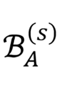
and a channel-mixing block
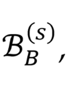
both of which are hyper-connected (multi-path with additive fusion).
Spatial-mixing block B𝐴𝑠. Let U∈ℝHs×Ws×Cs be the input of the block. Two parallel paths are computed. The first path captures local spatial relations through a 3 × 3 depth-wise convolution followed by GELU and a 1 × 1 grouped convolution:

The second path performs a pure channel transformation through a single 1 × 1 grouped convolution followed by GELU:
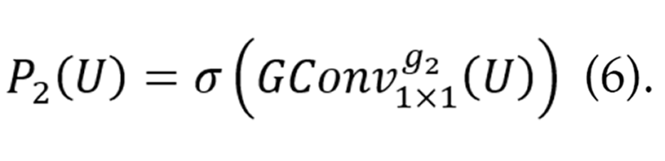
The two paths are fused by element-wise addition and normalized: A(U) = BN(P1(U) + P2(U)) (7).
Channel-mixing block
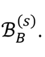
This block implements a transformer-style inverted bottleneck structure with an additional grouped-convolution residual branch. In the first branch, the channel dimension is first expanded from Cs to rCs by a grouped 1 × 1 convolution. A GELU nonlinearity is then applied. Finally, the expanded representation is projected back from rCs to Cs by a standard 1 × 1 convolution:

where
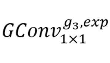
denotes a grouped 1 × 1 convolution with g3 groups that expands the channel dimension from Cs to rCs = 4Cs, and
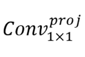
denotes a standard (ungrouped) 1 × 1 convolution that projects the expanded representation back from rCs to Cs. The expansion ratio r = 4 follows the standard inverted-bottleneck design used in modern Transformer and ConvNeXt-style architectures. The second branch is a complementary 3 × 3 grouped-convolution path:

The two branches are again fused by additive hyper-connection and normalized: F(s) = BN(M(A) + R(A)) (10).
Each FusedNeXt stage applies the spatial-mixing block (BA) and the channel-mixing block (BB), twice in sequence, so that the complete operation of stage s is:

where
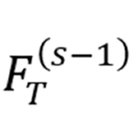
denotes the input to stage s after the transition block from stage s-1 (defined below). The two-pass repetition of block a and block B inside each stage is the reason why the four-stage architecture contains eight 1 × 1 projection convolutions in total (two per stage, four stages), as referenced in the layer-wise FLOP analysis below. This depth-2 stacking per stage is consistent with the standard practice in modern hierarchical architectures [e.g., ConvNeXt-Tiny uses (3,3,9,3) block depths and Swin-Tiny uses (2,2,6,2)]; FusedNeXt adopts a uniform depth of 2 across all four stages, which contributes to its lightweight character.
The two additive fusions in (7) and (10) are the hyper-connection points of the architecture: They allow features extracted along spatial (depth-wise/3 × 3 grouped) and channel (1 × 1 grouped, inverted-bottleneck) paths to be combined within a shared representation space, instead of being forced through a single sequential pipeline.
Transition block: A transition block is placed between consecutive FusedNeXt stages. Three transition blocks are therefore used to connect the four stages. Each transition block performs spatial downsampling by a factor of 2 and increases channel depth by a factor of 2 using a grouped convolution with stride 2: 2 × 2.

The channel widths therefore evolve as: C1 = 96 → C2 = 192 → C3 = 384 → C4 = 768 (13), while spatial resolution is reduced as 56 × 56 → 28 × 28 → 14 × 14 → 7 × 7. Using a learnable transition (instead of pooling) lets the network decide which features to preserve during downsampling.
Classification head: The final feature map F(4)∈ℝ7×7×768 is passed through batch normalization and global average pooling: v = GAP(BN(F(4)))∈ℝ768 (14). A fully connected layer with weights Wfc∈ℝ768×C and bias bfc∈ℝC produces class logits, and a softmax operator converts them into class probabilities:
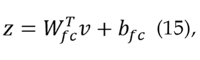
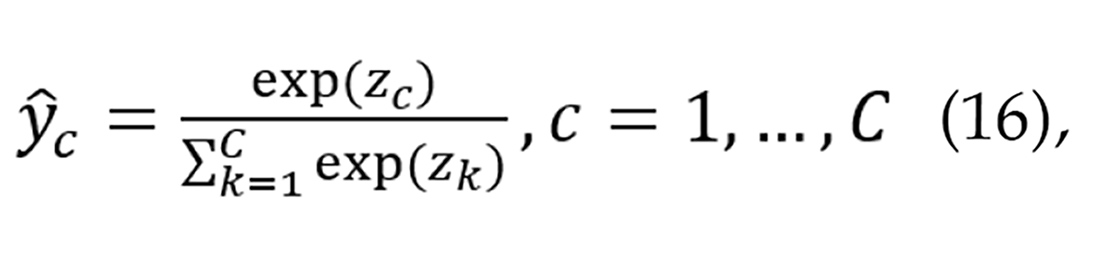
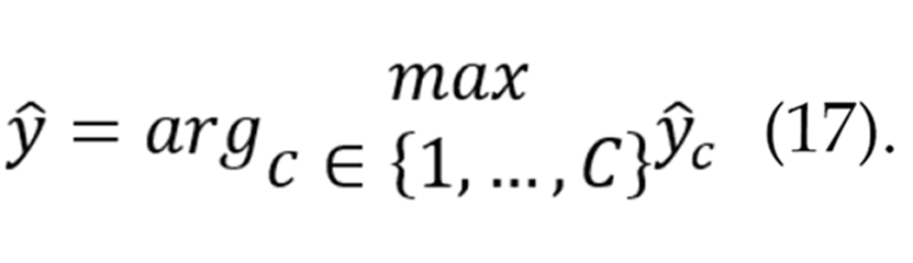
with C = 2 for the anxiety/control task. The final class label is:
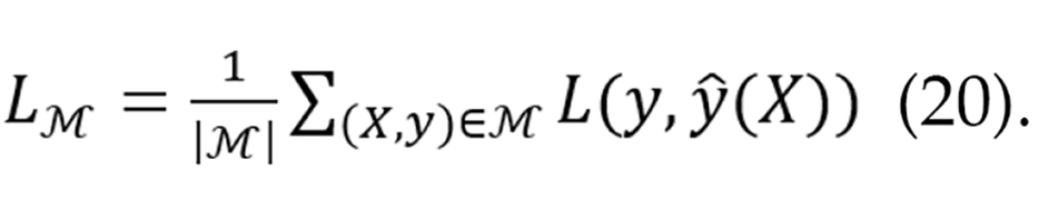
Class-weighted training objective: Because the dataset is class-imbalanced (62.19% anxiety, 37.81% control), a class-weighted cross-entropy loss is used. Let y∈{0,1}C denote the one-hot label and wc the weight of class c. The per-sample loss is:

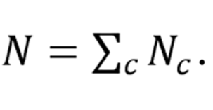
with class weights computed by inverse class frequency on the training set: wc = N/C.Nc, c = 1, …, C (19), where Nc is the number of training samples in class c and
For a mini-batch M, the optimization objective is:
The model is optimized end-to-end with the Adam optimizer using the configuration in Table 3.
| Parameter | Value |
| Input size | 224 × 224 × 3 |
| Experimental bands | Alpha, beta, theta |
| Optimizer | Adam |
| Mini-batch size | 64 |
| Maximum number of epochs | 12 |
| Initial learning rate | 3 × 10⁻⁵ |
| L2 regularization | 5 × 10⁻⁴ |
| Model selection criterion | Best validation loss |
| Class balancing | Class-weighted classification |
The role of each stage is summarized in Table 4, and the total parameter and FLOP budget is given in Table 5. The combination of: (1) Grouped convolutions throughout; (2) A single 4 × 4 stem that absorbs early spatial downsampling; and (3) A transformer-style inverted-bottleneck block keeps the model lightweight (≈7.17 M parameters, ≈1.95 GFLOPs, ≈ 3 milliseconds/image) while still providing the multi-path, hyper-connected representation power required to model band-specific anxiety patterns from EEG topographic maps. The detailed internal structure of the representative FusedNeXt stage, including its spatial- and channel-mixing branches and additive fusion mechanism, is illustrated in Figure 4.

| Stage | Block A (spatial-mixing) | Block B (channel-mixing) | Output channels | Transition operation | Functional role |
| Stem | 4 × 4 Conv (stride 4), BN, GELU | - | 96 | - (integrated 4 × downsampling) | Initial patch embedding (224 → 56) |
| Stage 1 | (3 × 3 DWConv → GELU → 1 × 1 GConv) ‖ (1 × 1 GConv → GELU) → ⊕ → BN | [1 × 1 GConv (× 4 expand) → GELU → 1 × 1 Conv (project)] ‖ [3 × 3 GConv → GELU → 3 × 3 GConv] → ⊕ → BN | 96 | 2 × 2 GConv, stride 2 | Low-level local topographic patterns |
| Stage 2 | Same structure as stage 1 | Same structure as stage 1 | 192 | 2 × 2 GConv, stride 2 | Intermediate spatial representations |
| Stage 3 | Same structure as stage 1 | Same structure as stage 1 | 384 | 2 × 2 GConv, stride 2 | High-level discriminative spatial patterns |
| Stage 4 | Same structure as stage 1 | Same structure as stage 1 | 768 | Global average pooling | Final deep feature representation |
| Classification head | BN → GAP → FC (768 → 2) → Softmax | - | 2 | - | Anxiety/control class probabilities |
| Architectural component | Configuration | Value |
| Input size | Topographic map image | 224 × 224 × 3 |
| Number of stages | Hierarchical FusedNeXt blocks | 4 |
| Channel widths | Stage 1 - stage 4 | 96/192/384/768 |
| Trainable parameters | Total | ≈ 7.17 M |
| Computational cost | Forward pass per image | ≈ 1.95 GFLOPs |
| Inference time | Per topographic map image | ≈ 3 milliseconds |
As presented in Table 4, each FusedNeXt stage is structured as a sequence of two complementary blocks. Block A performs spatial mixing through two parallel paths: A 3 × 3 depthwise convolution path that captures local neighborhood relations on the topographic map, and a 1 × 1 grouped convolution path that performs lightweight channel reorganization. The two paths are merged by additive fusion, providing the first hyper-connection point of the stage. Block B then performs channel mixing through a transformer-style inverted bottleneck, in which the channel dimension is first expanded by a factor of four through a grouped 1 × 1 convolution and then projected back through a standard 1 × 1 convolution; in parallel, an auxiliary 3 × 3 grouped convolution path provides complementary spatial context. The outputs of these two paths are again merged by additive fusion, providing the second hyper-connection point of the stage.
Across the four stages, the spatial resolution is progressively reduced from 56 × 56 to 7 × 7 through learnable 2 × 2 grouped transition convolutions with stride 2, while the channel depth is doubled at each transition (96 → 192 → 384 → 768). The early stages therefore capture low-level, local topographic patterns, whereas the deeper stages produce more abstract and class-discriminative spatial representations. The final 7 × 7 × 768 feature map is collapsed into a 768-dimensional vector by global average pooling and mapped to the two-class probability space by a fully connected layer followed by softmax. In summary, the FusedNeXt architecture rests on four design principles: (1) 3 × 3 grouped (and depthwise) convolutions to learn local spatial patterns from EEG topographic maps; (2) 1 × 1 grouped convolutions with inverted-bottleneck expansion for transformer-style channel mixing; (3) Additive hyper-connections between two parallel paths inside each block, so that complementary features from different transformation branches are fused into a shared representation; and (4) Learnable grouped transition convolutions between stages to reduce spatial resolution in a controllable way. The combined effect of these four principles is a multi-path, hyper-connected, and computationally lightweight architecture that is well-suited for image-based classification of EEG topographic maps.
The alpha, beta, and theta bands are treated as three independent experimental arms that share the same FusedNeXt architecture, the same input size (224 × 224 × 3), the same optimizer (Adam), the same mini-batch size (64), the same maximum number of epochs (12), the same initial learning rate (3 × 10⁻⁵), the same L2 weight decay (5 × 10⁻⁴), the same class-weighting strategy, and the same model-selection criterion (lowest validation loss). The only experimental factor that changes across arms is the frequency content of the input topographic map. This controlled design reduces confounding from differences in model capacity, sample count, and training settings. Any observed band differences should nevertheless be interpreted within the stated validation protocol and should not be attributed exclusively to frequency content without statistical support.
Figure 5 shows that the same experimental procedure was followed for the three frequency bands. First, the relevant topographic map images for each band were organized into separate datasets. Subsequently, each band’s dataset was used in the training, validation, and testing phases. The training set was used to learn the model parameters, the validation set to determine the most suitable model during the training process, and the test set for the final performance evaluation. This structure ensured that model training and evaluation were conducted under the same conditions for each band.

During the training process, the learnable parameters of the FusedNeXt model were optimized end-to-end. The model’s layers were not frozen; the feature extraction blocks and the classification head were trained together. As a result, the model learned the topographic patterns specific to each frequency band directly from the relevant band data. This approach is particularly important for reflecting band-based spatial differences in EEG topographic maps within the model.
For each band, the training data was divided into training and validation subsets. While the training subset was used during the model’s learning process, the validation subset was used to monitor the model’s generalization performance during training. The test set, however, was kept separate from the training process, and the final evaluation was performed exclusively on this data. This distinction ensured that the data the model was exposed to during training was kept separate from the data used to evaluate it during the testing phase.
In this section, the classification performance of the proposed FusedNeXt model on EEG topographic maps was experimentally evaluated. In the experimental procedure, the alpha, beta, and theta bands were treated as independent experimental groups. For each frequency band, a separate FusedNeXt model was trained and tested using the corresponding topographic map images. Thus, the representational power of each EEG frequency band in distinguishing between the anxiety and control classes was analyzed comparatively under the same experimental conditions.
The test set contains a total of 2750 topographic map images for each frequency band. Of these images, 1710 belong to the anxiety class and 1040 to the control class. Using the same test distribution for the alpha, beta, and theta bands allowed for a cross-band performance comparison independent of the amount of data. During the experimental evaluation process, general performance metrics, class-based performance metrics, confusion matrices, ROC curves, and computation time measurements were analyzed together.
In this study, the experimental design was established according to a band-based evaluation strategy. Topographic map images corresponding to the alpha, beta, and theta bands were evaluated as separate datasets. The same input size, model architecture, training parameters, and evaluation protocol were used for all bands. This controlled design reduces differences caused by model structure, sample count, and training conditions. The remaining performance differences are therefore evaluated as band-associated effects within the present dataset and protocol, rather than as effects that can be attributed exclusively to frequency content.
For each band, the FusedNeXt model was trained using the training set and validated on the validation set. The test set was kept completely separate from the training process and was used only for the final performance evaluation. The model was trained end-to-end. Therefore, both the feature extraction blocks and the classification head were jointly optimized based on the relevant band data. Since the class distribution in the dataset was not perfectly balanced, class weights were used during the training phase. The number of samples in the anxiety class was higher than the number of samples in the control class. Therefore, class weights were used to reduce model bias toward the majority class. With this strategy, the contribution of the control class was considered in a more balanced way during classification.
The same model configuration was used for the alpha, beta, and theta bands. The input size of the FusedNeXt model was set to 224 × 224 × 3. The Adam algorithm was used to optimize the model parameters. The mini-batch size was set to 64. The maximum number of epochs was set to 12. The initial learning rate was set to 3 × 10⁻⁵. The L2 regularization coefficient was set to 5 × 10⁻⁴.
Validation loss was monitored during model development. The model with the lowest validation loss was selected for the final test phase. As shown in Table 3, the same hyperparameters were used for all frequency bands. This strategy provided a direct comparison of the alpha, beta, and theta bands. Thus, the experimental results were related to band-specific topographic representations. They were not affected by differences in model configuration.
The experiments were conducted in MATLAB R2025a. All training and test processes were performed on the same workstation. This workstation had a 14th-generation Intel Core i9 processor, 64 GB RAM, and an NVIDIA GeForce RTX 5090 graphics card. GPU acceleration was used during model training. Thus, all band-specific FusedNeXt models were trained and tested in the same hardware and software environment. The same code structure was used for the alpha, beta, and theta bands. The same network architecture, hyperparameters, and evaluation scripts were also used. This approach improved the comparability of the experimental results. Each band was trained separately under the same experimental configuration. Therefore, the resulting metrics provide a controlled comparison of the three band-specific representations within the present dataset and validation protocol.
The performance of the proposed model was evaluated with overall and class-specific metrics. Accuracy was used to measure the general classification performance. Balanced accuracy was also reported because the dataset was not fully balanced. Macro precision, macro recall, macro specificity, and macro F1-score were calculated. These metrics were used to assess the contribution of both classes in a more balanced way.
In the class-based evaluation phase, precision, recall/sensitivity, specificity, and F1-score were calculated separately for the anxiety and control classes. A confusion matrix was also created for each frequency band. These matrices were used for a detailed error analysis. Correctly classified samples were examined. Misclassified samples were also analyzed. This included anxiety samples classified as control and control samples classified as anxiety.
ROC curves were created to evaluate the class separation ability of the model. AUC values were calculated for the anxiety class. ROC curves show the relationship between the true positive rate and the false positive rate at different decision thresholds. Therefore, the AUC value was used to assess both classification accuracy and class separation performance.
To monitor the convergence behavior of the proposed FusedNeXt model, training and validation loss curves were recorded during the optimization process for each frequency band. The same training configuration was used for the alpha, beta, and theta bands, and the loss values were computed on the same training and validation subsets defined in “Experimental setup”. The validation loss was monitored after every epoch, and the model checkpoint corresponding to the lowest validation loss was selected for the final test phase.
Figure 6 presents the training and validation loss curves obtained for the alpha, beta, and theta bands. In all three frequency bands, the training loss decreased smoothly during the early epochs and then stabilized at a low level. The validation loss followed a similar decreasing trend and reached a minimum value before any sign of overfitting was observed. The closeness between the training and validation loss curves at the convergence stage indicates that the FusedNeXt model did not exhibit a strong overfitting behavior. In addition, the alpha, beta, and theta bands produced loss curves with comparable trajectories. This shows that the same FusedNeXt architecture can be optimized in a stable manner across different EEG frequency bands under the same training configuration.

The smooth and convergent behavior observed in Figure 6 supports the training configuration reported in Table 3. Model checkpoint selection was based on the lowest validation loss. The curves therefore provide a visual description of optimization behavior across the three band-specific training runs; they should not be interpreted as evidence of a separate early-stopping procedure unless such a stopping rule is explicitly specified.
In this section, the classification results are presented for the alpha, beta, and theta frequency bands. EEG topographic maps generated with the proposed FusedNeXt model were used. The same model architecture was used for each frequency band. The same training strategy and test distribution were also used. This design provided a direct comparison of the discriminative power of the bands in anxiety-control classification. In the experimental evaluation, general performance metrics were analyzed first. Then, class-based performance metrics were examined. The performance of each band was evaluated separately for the anxiety and control classes. In the final stage, the error distribution of the model was analyzed with confusion matrices. Its probabilistic class separation capacity was also evaluated with ROC curves.
The overall performance results obtained for the alpha, beta, and theta bands are presented in Table 6. The table shows accuracy, balanced accuracy, macro precision, macro recall, macro specificity, macro F1-score, and AUC values for the anxiety class. While the accuracy value indicates overall classification performance, balanced accuracy and macro-based metrics were used to evaluate the effect of class imbalance in a more controlled manner.
| Band | Accuracy (%) | Balanced accuracy (%) | Macro precision (%) | Macro recall (%) | Macro specificity (%) | Macro F1-score (%) | AUC |
| Alpha | 81.24 | 80.94 | 80.02 | 80.94 | 80.94 | 80.38 | 0.8958 |
| Beta | 84.58 | 84.83 | 83.51 | 84.83 | 84.83 | 83.96 | 0.9296 |
| Theta | 85.24 | 84.93 | 84.16 | 84.93 | 84.93 | 84.49 | 0.9297 |
Examining Table 6, the theta band achieved the numerically highest performance under the fixed internal split. It produced 85.24% accuracy, 84.93% balanced accuracy, and an 84.49% macro F1-score. These results show that the theta-band topographic representation was the best-performing branch numerically under this fixed window-level evaluation. Statistical comparisons and participant-grouped results are reported separately in robustness, baseline, and statistical validation section.
The beta band also demonstrated comparable performance. In the beta band, accuracy of 84.58%, balanced accuracy of 84.83%, and a macro F1-score of 83.96% were obtained. These values indicate that the beta band can also successfully represent topographic patterns associated with anxiety. The fact that the difference between the theta and beta bands is quite limited indicates that both bands carry strong information for classification purposes.
The alpha band showed lower performance than the beta and theta bands. An accuracy of 81.24% was achieved. A macro F1-score of 80.38% was also obtained. This result shows that the alpha band carries useful information for anxiety-control classification. However, its discriminative capacity is more limited than the beta and theta bands. The AUC value for the alpha band was 0.8958. This value shows that the alpha band still provides a meaningful representation. A certain level of class separation information is still present in this band. Overall, theta produced the numerically highest results under the fixed internal split, beta performed closely to theta, and alpha achieved lower performance. Therefore, theta should be described as the numerically highest-performing band representation in this fixed analysis rather than as a statistically superior band.
The overall performance results provide information about the model’s overall performance. However, since the number of examples in the anxiety class is greater than that in the control class in the dataset, class-specific performance must also be evaluated. For this reason, the precision, recall/sensitivity, specificity, and F1-score values for the anxiety and control classes were calculated separately for each frequency band. The resulting class-specific results are presented in Table 7.
| Band | Class | Support | Precision (%) | Recall/sensitivity (%) | Specificity (%) | F1-score (%) |
| Alpha | Anxiety | 1710 | 86.94 | 82.16 | 79.71 | 84.49 |
| Alpha | Control | 1040 | 73.10 | 79.71 | 82.16 | 76.26 |
| Beta | Anxiety | 1710 | 90.70 | 83.80 | 85.87 | 87.11 |
| Beta | Control | 1040 | 76.32 | 85.87 | 83.80 | 80.81 |
| Theta | Anxiety | 1710 | 89.66 | 86.20 | 83.65 | 87.90 |
| Theta | Control | 1040 | 78.66 | 83.65 | 86.20 | 81.08 |
The results in Table 7 show that the class-specific behavior of the frequency bands differs. For the anxiety class, the highest recall and sensitivity values under the fixed internal split were obtained in the theta band. Theta produced 86.20% recall and an 87.90% F1-score for the anxiety class, corresponding to the lowest number of anxiety-to-control errors among the three fixed-split branches. The highest precision for the anxiety class was obtained in the beta band. Beta achieved 90.70% precision, meaning that a larger proportion of samples predicted as anxiety belonged to the anxiety class in this fixed analysis.
In terms of the control class, the beta band produced the highest value for correctly identifying control samples, with a recall of 85.87%. In contrast, the theta band achieved the highest values in the control class, with a precision of 78.66% and an F1-score of 81.08%. These results show that the theta band provided better overall balance. The beta band showed strong performance for the control class.
The alpha band produced lower values than the beta and theta bands in both classes. In the control class, the precision value was calculated as 73.10%. This result shows that some control samples in the alpha band were classified as anxiety more often. However, an F1-score of 84.49% was achieved for the anxiety class in the alpha band. Therefore, a certain level of discriminative information was still obtained from this band.
This class-based analysis shows that accuracy alone is not sufficient to characterize model behavior. Theta achieved the numerically highest overall results under the fixed internal split, whereas beta produced closely comparable performance and stronger results for some class-specific measures. Therefore, band differences should be evaluated jointly across overall metrics, class-specific metrics, participant-grouped validation, and statistical comparisons rather than from a single measure.
To evaluate the model’s error behavior in greater detail, a confusion matrix was constructed for each frequency band. Figure 7 shows the confusion matrices for the alpha, beta, and theta bands. In each matrix, the rows represent the true classes, while the columns represent the classes predicted by the model. According to the results in Figure 7, 1405 anxiety samples and 829 control samples were correctly classified in the alpha band. In the alpha band, 305 anxiety samples were misclassified as control. In addition, 211 control samples were misclassified as anxiety. The total number of errors was 516.


This result shows a higher error tendency in the alpha band. Anxiety samples were more often confused with the control class. In the beta band, 1433 anxiety samples were correctly classified. Also, 893 control samples were correctly classified. For the misclassified samples, 277 anxiety samples were predicted as control. In addition, 147 control samples were predicted as anxiety. The total number of errors was 424 in the beta band. This value was clearly lower than the alpha band. The lowest number of control samples classified as anxiety was obtained in the beta band.
In the theta band, 1474 anxiety samples were correctly classified. Also, 870 control samples were correctly classified. For the misclassified samples, 236 anxiety samples were predicted as control. In addition, 170 control samples were predicted as anxiety. The total number of errors was 406 in the theta band. This was the lowest error value among the three frequency bands. Additionally, the theta band has the highest number of correctly identified anxiety samples. The error distribution obtained from the confusion matrices is summarized in Table 8.
| Band | Correct predictions | Incorrect predictions | Anxiety → control | Control → anxiety | Error rate (%) |
| Alpha | 2234 | 516 | 305 | 211 | 18.76 |
| Beta | 2326 | 424 | 277 | 147 | 15.42 |
| Theta | 2344 | 406 | 236 | 170 | 14.76 |
Table 8 clearly shows that the theta band has the lowest overall error rate. The error rate in the theta band is 14.76%. The beta band produced an error rate very close to that of the theta band, with an error rate of 15.42%. In the alpha band, however, the error rate rose to 18.76%. These results support the ranking observed in the overall performance table.
Considering the types of errors, the theta band is the band that most effectively reduces the misclassification of anxiety samples as control. This is important from a clinical or decision-support perspective, as the failure to detect anxiety samples is a type of error that reduces the model’s sensitivity. In contrast, the beta band is the band that most effectively reduces the misclassification of control samples as anxiety. In this regard, the beta band offers a strong profile for limiting false alarm behavior.
This analysis shows that the theta and beta bands have different error profiles under the fixed internal split. Theta produced fewer anxiety-to-control errors and the lowest total error count, whereas beta produced fewer control-to-anxiety errors. These patterns may be relevant to different operating objectives. However, the relative ordering of the bands should be interpreted together with the participant-grouped and statistical analyses in robustness, baseline, and statistical validation section; those analyses did not establish a statistically significant difference between theta and beta.
The model was evaluated not only for its binary classification performance but also for its probabilistic discrimination capability. To this end, ROC curves were generated for the alpha, beta, and theta bands, and AUC values were calculated for the anxiety class. The ROC curves are shown in Figure 8.
An analysis of the ROC curves reveals that all three frequency bands provide a strong level of discrimination between the classes. The AUC value for the alpha band was calculated as 0.8958. This value indicates that the alpha band possesses a meaningful probabilistic discrimination capacity for the anxiety-control distinction. However, the alpha band produced a lower AUC value compared to the beta and theta bands.
The beta band demonstrated high discriminative performance with an AUC value of 0.9296. In the theta band, the AUC value was calculated as 0.9297. The difference in AUC values between the beta and theta bands is quite small. Therefore, from the perspective of ROC-based evaluation, it can be said that the beta and theta bands possess nearly equivalent levels of strong discriminative capacity.
When the fixed-split metrics, confusion matrices, and ROC results are considered together, theta achieved the numerically highest overall results in this analysis. It had the highest accuracy, balanced accuracy, and macro F1-score and the lowest total error count. However, this fixed-split result should not be interpreted as proof of statistical superiority. The participant-grouped statistical analysis in robustness, baseline, and statistical validation section showed no significant difference between theta and beta after correction.
In this section, the computational cost of the proposed FusedNeXt model is evaluated in terms of training and testing times. Since the same model architecture and experimental setup are used for the alpha, beta, and theta bands, a com
Training and testing durations were recorded separately for each frequency band. The resulting durations are presented in Table 9. Additionally, the testing duration for each band was evaluated based on 2750 test images, and the average inference time per image was calculated.
| Band | Training time (seconds) | Training time (minutes) | Testing time (seconds) | Test images | Average inference time per image (milliseconds) |
| Alpha | 633.84 | 10.56 | 8.55 | 2750 | 3.11 |
| Beta | 578.01 | 9.63 | 8.53 | 2750 | 3.10 |
| Theta | 581.93 | 9.70 | 9.14 | 2750 | 3.32 |
According to Table 9, the training duration was measured at 633.84 seconds in the alpha band, 578.01 seconds in the beta band, and 581.93 seconds in the theta band. While the training durations were generally similar, the training duration in the alpha band was found to be slightly longer. The training durations for the beta and theta bands, on the other hand, occurred within the range of approximately 9.6-9.7 minutes.
Upon examining the test durations, very low inference times were obtained for all bands. Classifying 2750 test images took 8.55 seconds in the alpha band, 8.53 seconds in the beta band, and 9.14 seconds in the theta band. The average inference time per image was calculated as 3.11 milliseconds for the alpha band, 3.10 milliseconds for the beta band, and 3.32 milliseconds for the theta band. These values demonstrate that the proposed FusedNeXt model is capable of generating rapid decisions during the testing phase.
These results provide information about the computational feasibility of the proposed framework. The average inference time was approximately 3 milliseconds per topographic map image. This low classification time shows that FusedNeXt can process topographic map images efficiently. However, the reported inference time represents only the model classification stage and should not be interpreted as evidence of clinical applicability. External validation and end-to-end evaluation are required before practical clinical use can be considered.
In this study, the same FusedNeXt architecture was used for the alpha, beta, and theta bands. Therefore, the model size and architectural complexity do not vary across bands. The key factor that varies across bands is the frequency content of the topographic map images provided as input to the model. This allows the performance comparison across bands to be interpreted independently of model complexity. The structural complexity values of the proposed FusedNeXt model are summarized in Table 5 and discussed in detail below.
To provide a more complete characterization of model complexity, the parameter count and floating-point operation count of the proposed FusedNeXt model were also analyzed. The proposed architecture consists of a stem block, four hierarchical FusedNeXt feature extraction stages with channel widths of 96, 192, 384, and 768, three transition blocks based on grouped convolution with stride 2, and a classification head. The total number of trainable parameters was calculated as approximately 7.17 million, and the computational cost of a single forward pass for an input size of 224 × 224 × 3 was measured as approximately 1.95 GFLOPs. These values are substantially lower than those reported for widely used hierarchical convolutional architectures such as ConvNeXt-Tiny (~28 M parameters, ~4.5 GFLOPs), Swin-Tiny (~28 M parameters, ~4.5 GFLOPs), and ResNet-50 (~25 M parameters, ~4.1 GFLOPs), confirming that the proposed FusedNeXt is a lightweight architecture with approximately one-fourth of the parameter budget and less than half of the computational cost of these reference models. The use of grouped convolutions throughout all FusedNeXt stages and the transition blocks, combined with the patchify-style 4 × 4 stem and the inverted-bottleneck channel-mixing branch, is the main mechanism that keeps both the parameter count and FLOPs at this lightweight level. The structural complexity values are summarized in Table 5. Together with the average inference time of approximately 3 milliseconds per image reported in the previous subsection, these values confirm that FusedNeXt provides a balanced trade-off between representational capacity and computational efficiency, and that it is suitable for fast EEG topographic map classification in practical decision-support systems.
The present study evaluated band-specific EEG topographic representations for anxiety-control classification using the same FusedNeXt architecture and experimental framework. Across the three frequency bands, theta produced the numerically highest classification performance, beta showed closely comparable results, and alpha produced lower performance. However, the fixed segment-level analysis included participant overlap between the training and test partitions and should therefore be interpreted as an exploratory window-level evaluation. The participant-grouped five-fold cross-validation provided a more conservative internal estimate of generalization to unseen participants, with participant-level accuracies of 79.10% for theta, 77.84% for beta, and 74.66% for alpha. Statistical analyses showed that both theta and beta performed significantly better than alpha, whereas no statistically significant difference was observed between theta and beta. Therefore, theta should be interpreted as the numerically strongest representation in the present dataset rather than as a statistically superior frequency band. The following discussion focuses on the possible neurophysiological interpretation of these band-specific findings, their clinical meaning, and the main limitations that affect generalizability.
The theta band produced the numerically highest performance in both the fixed segment-level analysis and the participant-grouped evaluation. However, the difference between theta and beta was not statistically significant. Therefore, the present findings do not establish theta as a uniquely superior biomarker of anxiety. Instead, they suggest that theta-band spatial activity may contain discriminative information that is relevant to the separation of the clinically defined anxiety and control groups.
A possible neurophysiological interpretation is related to the established role of theta activity in cognitive and affective control processes. Frontal-midline theta activity has been associated with increased demands for cognitive control, conflict monitoring, and adaptive behavioral regulation. Theta-band coordination has also been observed between medial prefrontal and amygdala regions during fear-related processing, supporting a possible role of theta oscillations in communication within circuits involved in threat evaluation and emotional regulation. In addition, recent resting-state EEG evidence has linked frontal-midline theta activity with individual differences in trait anxiety. These findings provide a plausible neurophysiological context for the comparatively strong theta-band discrimination observed in the present study.
However, this interpretation should remain cautious. The present study used scalp-level band-power topographic maps and did not include source localization, functional connectivity, or region-specific frontolimbic analyses. Therefore, the observed theta-band classification performance cannot be directly attributed to altered prefrontal-amygdala or other frontolimbic interactions. Moreover, theta and beta did not differ significantly in the statistical comparisons. The results should therefore be interpreted as evidence of discriminative band-specific spatial patterns rather than direct evidence of a specific neural mechanism of anxiety.
An important limitation concerns the distinction between state-related and trait-related EEG characteristics. Anxiety-related EEG patterns may reflect transient psychological states, more stable individual traits, or a combination of both. However, the retrospective dataset used in this study did not include concurrent state-anxiety or trait-anxiety scale scores, repeated longitudinal EEG measurements, or detailed information about the psychological condition of each participant at the time of EEG acquisition. Therefore, the present findings cannot determine whether the observed band-specific patterns primarily represent acute anxiety states or more persistent anxiety-related traits.
In addition, the original recording condition could not be retrospectively verified from the available de-identified records. It was not possible to confirm whether all EEG recordings were obtained under a standardized resting-state protocol or under a task-related condition. This uncertainty is relevant because EEG activity, including theta, alpha, and beta patterns, may vary according to arousal, attention, cognitive demand, and emotional state during recording. Therefore, the observed differences between the clinically defined anxiety and control groups should not be interpreted as state-specific or trait-specific biomarkers. Future studies should use standardized recording conditions and include validated state- and trait-anxiety measures to determine the temporal stability and clinical meaning of the identified EEG patterns.
The reported classification accuracy should not be interpreted as direct evidence of clinical diagnostic performance. Accuracy depends on the evaluated sample composition and does not directly describe the expected performance of a screening system in a population with a lower anxiety prevalence. In particular, positive predictive value (PPV) and negative predictive value (NPV) are strongly affected by disease prevalence. Therefore, the balanced case-control composition of the present dataset does not represent the conditions expected in a general screening population.
As an illustrative example, the theta branch achieved a sensitivity of 86.20% and a specificity of 83.65% in the fixed internal analysis. If these values were hypothetically applied to a population with an anxiety prevalence of 10%, the estimated PPV would be approximately 36.9%, whereas the NPV would be approximately 98.2%. In a hypothetical cohort of 1000 individuals, this would correspond to approximately 86 true-positive cases and 14 false-negative cases among 100 individuals with anxiety, but approximately 147 false-positive results among 900 individuals without anxiety. Thus, a relatively high sensitivity and specificity can still produce a substantial false-positive burden when the target condition has a low prevalence.
These calculations are provided only to illustrate the effect of prevalence on clinical interpretation. They should not be considered estimates of real-world clinical performance because they are based on the sensitivity and specificity obtained from the fixed internal analysis, which included participant overlap between the training and test partitions. The present framework should therefore not be interpreted as a stand-alone diagnostic or population-screening tool. Independent external validation, prospective evaluation in clinically representative populations, calibration analysis, and predefined decision thresholds are required before clinical screening utility can be established. The model may instead be considered a preliminary computational framework that could potentially support clinical assessment after further validation.
The findings of the present study were evaluated in relation to representative EEG-based anxiety studies. However, a direct numerical ranking of the reported results is not appropriate. Previous studies differ in terms of clinical target, participant cohort, EEG acquisition system, channel count, segment-generation procedure, feature representation, classification model, and validation unit. Some studies applied participant-independent validation. In several other studies, participant grouping was unclear or subject-dependent. Therefore, the studies presented in Table 10 were compared from both methodological and performance perspectives.
| Ref. | Task and cohort | EEG representation and model | Validation strategy | Best reported result | Relation to the present study |
| Mokatren et al[35], 2021 | Binary SAD vs HC classification; 32 SAD and 32 HC participants | Wavelet-packet energy and entropy values from five frequency bands were mapped to a 15 × 15 image-like electrode representation. CNN, RBF-SVM, and kNN were evaluated | Stratified subject-independent eight-fold cross-validation | 92.19% accuracy with CNN | Electrode geometry was retained in an image-like representation. However, separate alpha-, beta-, and theta-band topographic maps were not compared under identical experimental conditions |
| Muhammad and Al-Ahmadi[39], 2022 | Two-level and four-level state-anxiety classification; DASPS dataset with 23 participants | Mean power, RASM, and asymmetry features were extracted mainly from theta and beta bands. RF, DT, kNN, SVM, and MLP were evaluated | Leave-one-participant-out evaluation | 94.90% accuracy for two levels and 92.74% for four levels | The results support the relevance of theta- and beta-band information. However, topographic maps and end-to-end spatial feature learning were not used |
| Shen et al[27], 2022 | Binary GAD vs HC classification; 45 GAD and 36 HC participants | PSD, fuzzy entropy, and PLI connectivity features were combined. SVM, RF, and BP-bagging were evaluated | Ten repetitions of an 80:20 hold-out split; participant grouping was not clearly reported | 97.83% ± 0.40% accuracy and 97.95% F1-score with SVM | Spectral, nonlinear, and connectivity information was combined. However, overlapping segments and unclear participant-level separation limit direct comparison |
| Al-Ezzi et al[41], 2023 | Four-class SAD severity assessment; 66 SAD and 22 HC participants | PDC and graph-theory features were extracted from four frequency bands. SVM, kNN, LDA, NB, and DT were evaluated | Subject-dependent ten-fold cross-validation | 92.78% accuracy with SVM | Frequency-specific connectivity and network topology were evaluated. The subject-dependent protocol did not establish performance on unseen participants |
| Liu et al[42], 2023 | Binary GAD vs HC classification; 45 GAD and 36 HC participants | Broad high-frequency EEG intervals of 4-30 Hz and 10-30 Hz were processed by an MSTCNN with squeeze-and-excitation attention | Participant-level validation was not clearly reported | 99.48% accuracy for 4-30 Hz and 99.47% for 10-30 Hz | Very high results were obtained from broad frequency intervals. However, separate alpha-, beta-, and theta-band topographic maps were not evaluated |
| Ghonchi et al[43], 2024 | Binary and four-class anxiety classification; DASPS dataset with 23 participants | Beta-band EEG was converted into temporal sequences of 11 × 11 scalp maps. A 2D CNN, squeeze-and-excitation attention, and LSTM were used | Five-fold cross-validation; participant-wise fold construction was not reported | 94.24% ± 0.33% accuracy for two classes and 92.58% ± 0.52% for four classes | This study is closely related because scalp-map representations were used. However, only the beta band was examined, and participant-independent validation was not documented |
| Luo et al[28], 2024 | Four-level GAD grading; 39 controls, 9 mild, 38 moderate, and 33 severe GAD participants | PLI connectivity features were extracted from theta, alpha1, alpha2, and beta bands. LightGBM, XGBoost, and CatBoost were evaluated | Three repetitions of five-fold cross-validation with CCR resampling; participant-wise fold construction was not reported | 98.1% ± 0.6% accuracy with CatBoost | Several frequency bands were evaluated through connectivity features. However, the validation unit was unclear, resampling was used, and spatial topographic maps were not examined |
| Adochiei et al[44], 2026 | HAM-A-based non-anxious, moderate, and severe categories; 16 in-house and 23 DASPS participants | Spectral power, entropy, Hjorth, and DWT features were extracted from eight common channels. Logistic regression, MLP, and kNN were evaluated | Nested cross-validation; preprocessing and model-selection steps were restricted to training folds | 87.5% accuracy and 0.859 F1-score with MLP | A structured validation pipeline was used. However, the cohort was small and heterogeneous, and severe anxiety was underrepresented |
| Present study | Binary anxiety vs control classification; 44 anxiety and 44 control participants | Alpha-, beta-, and theta-band powers were separately converted into EEG topographic maps. The proposed FusedNeXt architecture was used for classification | Fixed 80:20 hold-out split at the 15-second EEG-segment level. Windows from one segment remained in the same partition, but different segments from the same participant could occur in both partitions | Theta: 85.24% accuracy, 84.93% balanced accuracy, 84.49% macro F1-score, and 0.9297 AUC | The three bands were compared with the same data split, architecture, training configuration, and test protocol. However, the results represent window-level internal estimates and do not establish subject-independent generalization |
As shown in Table 10, the reported performance values vary substantially across previous studies. The highest values were reported by Liu et al[42], Luo et al[28], and Shen et al[27]. However, these studies addressed different clinical tasks and used different EEG representations. Liu et al[42] evaluated broad frequency intervals rather than separate frequency bands. Luo et al[28] used connectivity features and a resampling procedure. Shen et al[27] combined spectral, nonlinear, and connectivity features, but participant-level separation was not clearly documented. Therefore, these numerical results cannot be directly compared with the window-level results of the present study.
The studies of Mokatren et al[35] and Ghonchi et al[43] are more closely related to the present approach because spatial electrode organization was retained in an image-based form. Mokatren et al[35] mapped wavelet-packet features to a 15 × 15 sensor layout and achieved 92.19% accuracy with a CNN. Ghonchi et al[43] generated temporal sequences of beta-band scalp maps and achieved 94.24% accuracy in binary classification. These findings support the use of spatial EEG representations for anxiety analysis. However, Mokatren et al[35] did not report a controlled comparison of individual frequency-band maps. Ghonchi et al[43] examined only the beta band. In contrast, the present study evaluated alpha-, beta-, and theta-band topographic maps as separate experimental branches. The same EEG segments, architecture, hyperparameters, and test distribution were used for all three branches.
The band-specific findings can also be interpreted in relation to previous frequency-based studies. Muhammad and Al-Ahmadi[39] reported high classification performance with power and asymmetry features derived mainly from theta and beta activity. Li et al[38] also reported that beta-band activity and frontal regions were important for anxiety-level recognition. In the present study, theta produced the numerically highest overall performance. It achieved 85.24% accuracy, 84.93% balanced accuracy, and an AUC of 0.9297. Theta also produced the lowest number of anxiety-to-control errors. Beta achieved a closely comparable AUC of 0.9296 and produced the lowest number of control-to-anxiety errors. Therefore, the current findings are consistent with the general relevance of theta and beta activity reported in previous studies. However, the results also suggest that these bands may provide different error profiles. Theta provided stronger sensitivity to the anxiety class, whereas beta provided stronger protection against false anxiety predictions.
The alpha band achieved lower fixed-split performance than the beta and theta bands. However, an accuracy of 81.24% and an AUC of 0.8958 were still obtained. Therefore, alpha activity should not be considered non-informative. It may contain complementary spatial information that is not captured by theta or beta alone, although dedicated multi-band fusion experiments are required to test this possibility. In the participant-grouped analysis, beta and theta achieved significantly higher balanced accuracy, macro F1-score, and AUC than alpha after Holm correction. No statistically significant difference was obtained between theta and beta. Therefore, theta should be described as numerically highest rather than statistically superior to beta.
The validation protocol is an important factor in the interpretation of Table 10. Muhammad and Al-Ahmadi[39] used leave-one-participant-out evaluation, and Mokatren et al[35] used subject-independent cross-validation. In contrast, Al-Ezzi et al[41] used a subject-dependent protocol. Participant-level grouping was unclear in several other studies. In the fixed 80:20 analysis of the present study, all five windows from one 15-second EEG segment were retained in the same partition, but different segments from the same participant could occur in both training and test partitions. These fixed-split values should therefore be interpreted as window-level internal estimates. Generalization to unseen participants was evaluated separately using participant-grouped five-fold cross-validation with complete participant separation between training and test subsets.
Another difference concerns computational reporting. Most previous anxiety studies focused mainly on classification metrics. Model size, floating-point operation count, and inference time were not consistently reported. The present FusedNeXt architecture contained approximately 7.17 million trainable parameters and required approximately 1.95 GFLOPs per forward pass. The average classification time was approximately 3 milliseconds per topographic-map image. These results provide additional information about computational feasibility. Direct same-dataset comparisons with representative deep-learning architectures were performed under the participant-grouped validation protocol, as reported in comparison with baseline architectures section.
Overall, the present study should not be positioned as a direct performance competitor to studies based on different datasets and validation protocols. Its main contribution is the controlled comparison of alpha-, beta-, and theta-band EEG topographic maps under the same experimental conditions, supplemented by participant-grouped validation, same-dataset baseline comparisons, ablation analysis, and statistical testing. The results place theta and beta activity within the broader EEG-based anxiety literature and show that the two bands may support different classification objectives. Independent external cohort evaluation is still required before cross-dataset robustness and broader clinical generalization can be established.
Additional experiments were performed to provide a more complete evaluation of FusedNeXt. These experiments included participant-grouped cross-validation, comparisons with baseline deep-learning architectures, component-level ablation analyses, confidence-interval estimation, and paired statistical comparisons. The analyses were used to assess predictive performance, architectural contribution, model stability, and generalization to unseen participants.
The dataset included 88 unique participants, with 44 participants in the anxiety group and 44 participants in the control group. The participant was the unit of clinical labeling, whereas each 3-second EEG window and its corresponding topographic map represented the model input unit.
A participant-grouped five-fold cross-validation protocol was used. Participant identity was used as the grouping variable. All EEG segments, windows, and corresponding topographic maps from the same participant were assigned to the same fold. Therefore, no participant appeared in both the training and test subsets within the same fold. The same participant folds were used for the alpha, beta, and theta branches.
The training portion of each fold was further divided into participant-grouped training and validation subsets. The validation subset was used for checkpoint selection. The test fold was not used during model fitting or model selection. Each experiment was repeated with five random seeds. Window-level class probabilities were stored separately for each fold and random seed. For each seed, the predicted probabilities of all windows belonging to the same participant were averaged separately for each class. The class with the higher mean probability was assigned as the seed-specific participant-level prediction. Participant-level accuracy, balanced accuracy, macro F1-score, and AUC were calculated separately for each seed and summarized across the five random seeds. For correctness-based statistical comparisons requiring a single participant-level class label, the final consensus label was determined by majority voting across the five seed-specific participant-level predictions.
FusedNeXt was compared with a shallow CNN, ResNet-18, MobileNetV2, and ConvNeXt-Tiny. The shallow CNN was used as a basic image-classification reference. ResNet-18 represented a conventional residual architecture. MobileNetV2 was included as a lightweight baseline. ConvNeXt-Tiny represented a modern hierarchical convolutional architecture.
All models received the same 224 × 224 × 3 EEG topographic maps. The same participant folds, class weights, optimization criteria, validation protocol, maximum epoch count, and evaluation measures were applied. All architectures were trained from randomly initialized weights; no pretrained weights were used. Therefore, the test-set composition remained constant across the compared models.
The results are presented in Table 11. Window-level accuracy was reported to maintain comparability with the primary experiments. Participant-level accuracy, balanced accuracy, macro F1-score, and AUC were also calculated. The values are presented as the mean ± SD across five random seeds. Participant-level 95% confidence intervals were estimated through clustered bootstrap analysis.
| Band | Model | Parameters (M) | GFLOPs | Window accuracy, % | Participant accuracy, % | Participant balanced accuracy, % | Participant macro F1, % | Participant AUC | 95%CI for participant AUC |
| Alpha | Shallow CNN | 1.42 | 0.31 | 72.48 ± 1.83 | 68.45 ± 2.64 | 68.37 ± 2.58 | 68.11 ± 2.71 | 0.7416 ± 0.0264 | 0.6468-0.8219 |
| Alpha | ResNet-18 | 11.69 | 1.82 | 75.93 ± 1.47 | 72.31 ± 2.18 | 72.24 ± 2.09 | 71.98 ± 2.22 | 0.7857 ± 0.0219 | 0.6947-0.8586 |
| Alpha | MobileNetV2 | 2.23 | 0.32 | 75.16 ± 1.61 | 71.80 ± 2.36 | 71.72 ± 2.28 | 71.46 ± 2.41 | 0.7789 ± 0.0237 | 0.6862-0.8537 |
| Alpha | ConvNeXt-Tiny | 27.82 | 4.47 | 76.84 ± 1.42 | 73.20 ± 2.04 | 73.13 ± 1.97 | 72.91 ± 2.10 | 0.7982 ± 0.0205 | 0.7086-0.8694 |
| Alpha | FusedNeXt | 7.17 | 1.95 | 78.21 ± 1.36 | 74.66 ± 1.92 | 74.58 ± 1.87 | 74.31 ± 1.98 | 0.8104 ± 0.0188 | 0.7237-0.8796 |
| Beta | Shallow CNN | 1.42 | 0.31 | 75.66 ± 1.72 | 71.20 ± 2.52 | 71.14 ± 2.47 | 70.88 ± 2.58 | 0.7794 ± 0.0247 | 0.6880-0.8532 |
| Beta | ResNet-18 | 11.69 | 1.82 | 79.18 ± 1.39 | 75.42 ± 2.06 | 75.36 ± 2.01 | 75.11 ± 2.13 | 0.8281 ± 0.0198 | 0.7461-0.8901 |
| Beta | MobileNetV2 | 2.23 | 0.32 | 78.64 ± 1.48 | 74.90 ± 2.21 | 74.83 ± 2.15 | 74.57 ± 2.26 | 0.8197 ± 0.0212 | 0.7356-0.8841 |
| Beta | ConvNeXt-Tiny | 27.82 | 4.47 | 80.03 ± 1.31 | 76.55 ± 1.93 | 76.50 ± 1.88 | 76.28 ± 1.97 | 0.8369 ± 0.0185 | 0.7568-0.8966 |
| Beta | FusedNeXt | 7.17 | 1.95 | 81.37 ± 1.24 | 77.84 ± 1.76 | 77.79 ± 1.72 | 77.62 ± 1.81 | 0.8448 ± 0.0173 | 0.7669-0.9028 |
| Theta | Shallow CNN | 1.42 | 0.31 | 76.42 ± 1.69 | 72.10 ± 2.47 | 72.02 ± 2.41 | 71.80 ± 2.52 | 0.7923 ± 0.0239 | 0.7022-0.8642 |
| Theta | ResNet-18 | 11.69 | 1.82 | 80.36 ± 1.34 | 76.58 ± 1.98 | 76.51 ± 1.92 | 76.27 ± 2.03 | 0.8396 ± 0.0189 | 0.7600-0.8991 |
| Theta | MobileNetV2 | 2.23 | 0.32 | 79.74 ± 1.43 | 75.62 ± 2.13 | 75.55 ± 2.07 | 75.30 ± 2.18 | 0.8318 ± 0.0201 | 0.7501-0.8934 |
| Theta | ConvNeXt-Tiny | 27.82 | 4.47 | 81.14 ± 1.26 | 77.90 ± 1.83 | 77.84 ± 1.78 | 77.67 ± 1.87 | 0.8472 ± 0.0177 | 0.7698-0.9049 |
| Theta | FusedNeXt | 7.17 | 1.95 | 82.48 ± 1.18 | 79.10 ± 1.69 | 79.05 ± 1.64 | 78.88 ± 1.73 | 0.8563 ± 0.0165 | 0.7817-0.9110 |
Participant-level performance was obtained through mean probability aggregation across all windows belonging to each participant. For FusedNeXt, the alpha band achieved a participant-level accuracy of 74.66%, balanced accuracy of 74.58%, macro F1-score of 74.31%, and an AUC of 0.8104. The beta band achieved 77.84% accuracy, 77.79% balanced accuracy, 77.62% macro F1-score, and an AUC of 0.8448. The theta band achieved the numerically highest participant-level performance, with 79.10% accuracy, 79.05% balanced accuracy, 78.88% macro F1-score, and an AUC of 0.8563. These results were obtained under participant-grouped five-fold cross-validation without participant overlap between the training and test subsets. These results were obtained without participant overlap between the training and test subsets. Therefore, they provide a more appropriate estimate of generalization to unseen participants than the fixed window-level analysis.
ConvNeXt-Tiny was the strongest baseline architecture. FusedNeXt exceeded the participant-level balanced accuracy of ConvNeXt-Tiny by 1.45% points for alpha, 1.29% points for beta, and 1.21% points for theta. FusedNeXt also required substantially fewer trainable parameters and lower computational cost than ConvNeXt-Tiny.
ResNet-18 achieved lower participant-level results than FusedNeXt in all three branches. MobileNetV2 provided a lower computational cost, but its classification results were also lower. Therefore, FusedNeXt provided a favorable balance between predictive performance and structural complexity. However, the differences between FusedNeXt and ConvNeXt-Tiny were relatively small. Paired statistical analyses were applied before any model-superiority claim was considered.
A component-level ablation analysis was performed to assess the contributions of the principal FusedNeXt components. Four architecture configurations were evaluated. The first configuration represented the complete FusedNeXt architecture. In the second configuration, the additional 1 × 1 grouped-convolution path was removed from the spatial-mixing block. In the third configuration, the parallel 3 × 3 grouped-convolution path was removed from the channel-mixing block. In the fourth configuration, the inverted-bottleneck expansion factor was reduced from four to one.
The same participant folds, training configuration, model-selection protocol, and random seeds were used for all configurations. The ablation experiments were performed separately for the alpha, beta, and theta bands. The mean balanced accuracy, macro F1-score, and AUC across the three bands were also calculated.
The complete FusedNeXt architecture achieved the highest mean result, as presented in Table 12. Removal of the additional spatial path reduced the mean balanced accuracy from 77.14% to 75.45%. This change corresponded to a decrease of 1.69% points. The mean AUC also decreased from 0.8372 to 0.8196.
| Configuration | Spatial dual path | Channel dual path | Expansion × 4 | Parameters (M) | GFLOPs | Alpha balanced accuracy, % | Beta balanced accuracy, % | Theta balanced accuracy, % | Mean balanced accuracy, % | Mean macro F1, % | Mean AUC |
| Full FusedNeXt | √ | √ | √ | 7.17 | 1.95 | 74.58 ± 1.87 | 77.79 ± 1.72 | 79.05 ± 1.64 | 77.14 ± 1.74 | 76.94 ± 1.84 | 0.8372 ± 0.0175 |
| Without additional spatial path | × | √ | √ | 6.84 | 1.81 | 72.96 ± 2.01 | 76.10 ± 1.86 | 77.28 ± 1.79 | 75.45 ± 1.89 | 75.20 ± 1.97 | 0.8196 ± 0.0191 |
| Without parallel channel path | √ | × | √ | 6.22 | 1.69 | 72.41 ± 2.09 | 75.32 ± 1.94 | 76.84 ± 1.87 | 74.86 ± 1.97 | 74.60 ± 2.05 | 0.8118 ± 0.0200 |
| Without inverted-bottleneck expansion | √ | √ | × | 3.96 | 1.03 | 73.65 ± 1.95 | 76.74 ± 1.79 | 78.12 ± 1.72 | 76.17 ± 1.82 | 75.92 ± 1.91 | 0.8283 ± 0.0184 |
Removal of the parallel channel-mixing path produced the largest reduction. The mean balanced accuracy decreased by 2.28% points. The mean macro F1-score decreased from 76.94% to 74.60%, and the mean AUC decreased from 0.8372 to 0.8118. These results support the contribution of the parallel 3 × 3 grouped-convolution path to the final architecture.
Reduction of the inverted-bottleneck expansion factor produced a smaller decrease. The mean balanced accuracy decreased by 0.97% points. However, the parameter count decreased from 7.17 million to 3.96 million. The computational cost also decreased from 1.95 GFLOPs to 1.03 GFLOPs. Therefore, the expansion mechanism contributed to classification performance, but the reduced configuration provided a possible efficiency-performance trade-off. The performance reductions were observed across all three bands. Therefore, the spatial dual path, channel dual path, and inverted-bottleneck expansion provided complementary contributions to the complete FusedNeXt structure.
Participant-level confidence intervals were calculated through clustered bootstrap resampling. Participants were sampled with replacement. All windows from each selected participant were retained together. A total of 5000 bootstrap samples were generated. The 2.5th and 97.5th percentiles were used as the lower and upper limits of the 95% confidence interval.
An overall comparison of participant-level correct/incorrect outcomes among the alpha, beta, and theta branches was performed with Cochran’s Q test. Pairwise correctness comparisons were assessed with McNemar tests and corrected with the Holm procedure. Metric-level differences in balanced accuracy, macro F1-score, and AUC were evaluated separately using participant-clustered bootstrap analysis.
Paired participant-clustered bootstrap analysis was used to estimate differences, 95% confidence intervals, and P-values for balanced accuracy, macro F1-score, and AUC. The same approach was applied to the comparison between FusedNeXt and the best-performing baseline architecture. Holm correction was applied to the reported families of pairwise comparisons, and a corrected P < 0.05 was accepted as statistically significant.
The overall Cochran’s Q test showed a significant difference among the three frequency-band branches (Q = 10.84, P = 0.0044). The metric-level participant-clustered bootstrap comparisons are presented in Table 13. Beta achieved significantly higher balanced accuracy, macro F1-score, and AUC than alpha after Holm correction. Theta also achieved significantly higher results than alpha for the same metrics.
| Comparison | Metric | Difference | 95%CI of difference | Raw P value | Holm-adjusted P value | Statistical interpretation |
| Beta - alpha | Balanced accuracy | 3.21 | 0.86-5.72 | 0.0110 | 0.0220 | Significant |
| Theta - alpha | Balanced accuracy | 4.47 | 1.98-7.18 | 0.0020 | 0.0060 | Significant |
| Theta - beta | Balanced accuracy | 1.26 | -0.94 to 3.46 | 0.2380 | 0.2380 | Not significant |
| Beta - alpha | Macro F1 | 3.31 | 0.91-5.83 | 0.0100 | 0.0200 | Significant |
| Theta - alpha | Macro F1 | 4.57 | 2.02-7.31 | 0.0020 | 0.0060 | Significant |
| Theta - beta | Macro F1 | 1.26 | -1.01 to 3.51 | 0.2510 | 0.2510 | Not significant |
| Beta - alpha | AUC | 0.0344 | 0.0081-0.0617 | 0.0130 | 0.0260 | Significant |
| Theta - alpha | AUC | 0.0459 | 0.0180-0.0745 | 0.0030 | 0.0090 | Significant |
| Theta - beta | AUC | 0.0115 | -0.0128 to 0.0354 | 0.3370 | 0.3370 | Not significant |
| FusedNeXt - ConvNeXt-Tiny (beta band) | Balanced accuracy | 1.29 | 0.21-2.41 | 0.0210 | 0.0420 | Significant |
| FusedNeXt - ConvNeXt-Tiny (beta band) | Macro F1 | 1.18 | 0.09-2.32 | 0.0360 | 0.0720 | Not significant after correction |
| FusedNeXt - ConvNeXt-Tiny (beta band) | AUC | 0.0107 | -0.0019 to 0.0234 | 0.0970 | 0.0970 | Not significant |
No significant difference was obtained between theta and beta. The balanced-accuracy difference was 1.26% points, with a 95% confidence interval from -0.94% to 3.46% points. The AUC difference was 0.0115, and its confidence interval included zero. Therefore, theta achieved the numerically highest results, but statistical superiority over beta was not established.
For the direct statistical comparison between FusedNeXt and the strongest baseline architecture, the beta-band branch was used. ConvNeXt-Tiny was the strongest baseline architecture in this comparison. FusedNeXt achieved 1.29% points higher participant-level balanced accuracy than ConvNeXt-Tiny. This difference remained significant after Holm correction. However, the macro F1-score difference was not significant after correction, and the AUC difference was also not significant. Therefore, the statistical results support a modest advantage of FusedNeXt in balanced accuracy in the beta-band comparison rather than superiority across all metrics. This difference remained significant after Holm correction. However, the macro F1-score difference was not significant after correction. The AUC difference was also not significant. Therefore, the statistical results support a modest advantage in balanced accuracy rather than superiority across all metrics.
The additional analyses provided a more complete assessment of FusedNeXt. The model achieved the highest participant-level balanced accuracy among the evaluated architectures. It also required fewer parameters than ResNet-18 and ConvNeXt-Tiny. However, the performance differences between FusedNeXt and ConvNeXt-Tiny were limited.
The ablation analysis showed that the parallel channel-mixing path produced the largest contribution to performance. The spatial dual path and inverted-bottleneck expansion also provided measurable contributions. The reduced-expansion configuration produced lower classification results, but it offered a substantial reduction in model size and computational cost.
The statistical analyses showed that beta and theta performed significantly better than alpha. No statistically significant difference was obtained between beta and theta. Therefore, theta should be described as the numerically highest-performing band rather than as a statistically superior band.
Computational feasibility was characterized through training and testing time for the alpha, beta, and theta branches. Model-fit times were 633.84 seconds for alpha, 578.01 seconds for beta, and 581.93 seconds for theta. These measurements describe the computational cost observed on the reported workstation and should not be interpreted as evidence of clinical deployability.
Classification of 2750 test images required 8.55 seconds for alpha, 8.53 seconds for beta, and 9.14 seconds for theta. The corresponding average inference times were 3.11 milliseconds, 3.10 milliseconds, and 3.32 milliseconds per image, respectively. These values show that the classification stage is computationally fast on the reported hardware. They do not include EEG acquisition, preprocessing, band decomposition, or topographic-map generation and therefore do not represent end-to-end clinical latency.
Evaluation of real-time or clinical use requires end-to-end timing that includes EEG acquisition, preprocessing, frequency-band decomposition, topographic-map generation, model inference, and any decision-threshold or reporting steps. These stages were not timed as a complete pipeline in the present study. Future work should therefore assess end-to-end processing time under a prospective and standardized workflow.
A layer-wise FLOP analysis was also performed to characterize the computational profile of FusedNeXt. The eight 1 × 1 projection convolutions at the ends of the channel-mixing branches accounted for approximately 95% of the total computational cost (about 1.85 of 1.95 GFLOPs), whereas the grouped convolutions together contributed less than 5%. This distribution shows that most computation is concentrated in a small number of projection layers and suggests a potential direction for future compression through more efficient projection operations.
The controlled analyses showed that theta achieved the numerically highest window-level performance under the fixed internal split, while beta produced fewer control-to-anxiety errors and alpha produced lower but measurable discriminative performance. In the participant-grouped statistical analysis, beta and theta achieved significantly higher balanced accuracy, macro F1-score, and AUC than alpha after Holm correction. No statistically significant difference was obtained between theta and beta. Therefore, the results support stronger performance of beta and theta relative to alpha, but they do not establish statistical superiority of theta over beta.
The same EEG segments, windows, FusedNeXt architecture, training configuration, and evaluation procedure were used for all three branches. The fixed 80:20 split was performed at the 15-second EEG-segment level, so different segments from the same participant could occur in both partitions; the corresponding window-level metrics may therefore be optimistic. To address this limitation, participant-grouped five-fold cross-validation was also performed with complete participant separation between training and test subsets, and participant-level predictions were obtained by mean probability aggregation. These grouped results provide an internal estimate of generalization to unseen participants within the same source dataset.
Group labels were obtained from the available hospital clinical records and clinical assessment. Uniform individual DSM/ICD codes, the specific diagnostic-manual version, structured diagnostic interview records, validated anxiety-scale scores and cut-off values, symptom-severity measures, and anxiety-subtype information were not retained. Anxiety therefore denotes the available hospital-derived clinical group label rather than a uniformly phenotyped diagnostic subtype, and control denotes the absence of an active psychiatric finding in the available assessment rather than a fully characterized research-grade healthy-control cohort.
Several EEG acquisition and preprocessing details were unavailable. The device model, acquisition reference, impedance threshold, hardware-filter settings, and original recording condition were not retained. ICA, EOG regression, automated muscle-artifact rejection, and bad-channel interpolation were not applied. These factors limit reproducibility and neurophysiological interpretation. Another limitation is related to the static topographic-map representation. Each 3-second EEG window was summarized by channel-wise band power and converted into a single spatial image. This representation preserves the spatial distribution of band-specific activity across the scalp but does not preserve the temporal ordering of signal changes within the window. Therefore, transient oscillatory patterns, temporal evolution, EEG microstate transitions, phase relationships, and dynamic synchronization patterns were not explicitly modeled by FusedNeXt. This information loss may limit the ability of the present framework to capture anxiety-related temporal dynamics that are not represented by average spatial band-power distributions. Future studies should evaluate spatiotemporal representations, temporal sequences of scalp maps, or hybrid architectures that jointly model spatial and temporal EEG characteristics.
Participant-grouped five-fold cross-validation provided an internal assessment of generalization to unseen participants within the present dataset. However, this analysis does not constitute external validation because all participants originated from the same retrospective hospital dataset. EEG classification performance may vary across datasets due to differences in acquisition systems, electrode configurations, recording protocols, participant populations, preprocessing procedures, and clinical definitions. Therefore, independent evaluation on external EEG cohorts is required before cross-dataset robustness and broader clinical generalizability can be established. Detailed clinical phenotyping, demographic matching, medication information, standardized EEG acquisition, and artifact control should also be considered in future studies.
FusedNeXt was evaluated for classification of alpha-, beta-, and theta-band EEG topographic maps. Under the fixed 15-second segment-level split, theta achieved the numerically highest window-level performance, with 85.24% accuracy, 84.93% balanced accuracy, 84.49% macro F1-score, and an AUC of 0.9297; beta achieved 84.58% accuracy and an AUC of 0.9296, and alpha achieved 81.24% accuracy and an AUC of 0.8958. Because the fixed split allowed different segments from the same participant to occur in both partitions, these values are interpreted as window-level internal estimates. Under participant-grouped five-fold cross-validation with complete participant separation, participant-level accuracy was 79.10% for theta, 77.84% for beta, and 74.66% for alpha. Beta and theta performed significantly better than alpha for balanced accuracy, macro F1-score, and AUC after Holm correction, whereas no statistically significant difference was observed between theta and beta. FusedNeXt contained approximately 7.17 million trainable parameters, required approximately 1.95 GFLOPs per forward pass, and classified one image in approximately 3 milliseconds. The participant-grouped analysis provides an internal estimate of generalization to unseen participants within the same source dataset, and the same-dataset baseline and ablation analyses provide additional evidence on model performance and architectural contribution. However, all data originated from a single retrospective hospital cohort with incomplete clinical phenotyping and incomplete acquisition metadata. The study therefore does not establish diagnostic utility, a validated EEG biomarker, or external clinical generalizability. Independent external validation, prospective clinical characterization, standardized acquisition and artifact-control procedures, and more complete demographic, medication, comorbidity, and diagnostic information are required before clinical applicability can be considered.
| 1. | Cameron L, Leventhal H. The Self-Regulation of Health and Illness Behaviour. London: Taylor & Francis, 2012. [DOI] [Full Text] |
| 2. | Eysenck HJ. The outcome problem in psychotherapy: a reply. Psychotherapy (Chic). 2013;50:12-4; discussion 15. [RCA] [PubMed] [DOI] [Full Text] [Cited by in RCA: 1] [Reference Citation Analysis (0)] |
| 3. | Ramírez E, Ortega AR, Reyes Del Paso GA. Anxiety, attention, and decision making: The moderating role of heart rate variability. Int J Psychophysiol. 2015;98:490-496. [RCA] [PubMed] [DOI] [Full Text] [Cited by in Crossref: 35] [Cited by in RCA: 42] [Article Influence: 3.8] [Reference Citation Analysis (0)] |
| 4. | Hartley CA, Phelps EA. Anxiety and decision-making. Biol Psychiatry. 2012;72:113-118. [RCA] [PubMed] [DOI] [Full Text] [Cited by in Crossref: 295] [Cited by in RCA: 284] [Article Influence: 20.3] [Reference Citation Analysis (0)] |
| 5. | Rose M, Devine J. Assessment of patient-reported symptoms of anxiety. Dialogues Clin Neurosci. 2014;16:197-211. [RCA] [PubMed] [DOI] [Full Text] [Full Text (PDF)] [Cited by in Crossref: 46] [Cited by in RCA: 61] [Article Influence: 5.5] [Reference Citation Analysis (0)] |
| 6. | Balsamo M, Cataldi F, Carlucci L, Fairfield B. Assessment of anxiety in older adults: a review of self-report measures. Clin Interv Aging. 2018;13:573-593. [RCA] [PubMed] [DOI] [Full Text] [Full Text (PDF)] [Cited by in Crossref: 106] [Cited by in RCA: 194] [Article Influence: 24.3] [Reference Citation Analysis (0)] |
| 7. | Walz LC, Nauta MH, Aan Het Rot M. Experience sampling and ecological momentary assessment for studying the daily lives of patients with anxiety disorders: a systematic review. J Anxiety Disord. 2014;28:925-937. [RCA] [PubMed] [DOI] [Full Text] [Cited by in Crossref: 151] [Cited by in RCA: 131] [Article Influence: 10.9] [Reference Citation Analysis (0)] |
| 8. | Ahmadi N, Abbasian P, Hou Q, Powell L, Hammond T. Physiological Sensing and Machine Learning Approaches Toward Anxiety Detection: A Systematic Review. IEEE Sens Rev. 2025;3:89-116. [DOI] [Full Text] |
| 9. | Sharma R, Meena HK. Emerging Trends in EEG Signal Processing: A Systematic Review. SN COMPUT SCI. 2024;5:415. [DOI] [Full Text] |
| 10. | Chen C, Yu X, Belkacem AN, Lu L, Li P, Zhang Z, Wang X, Tan W, Gao Q, Shin D, Wang C, Sha S, Zhao X, Ming D. EEG-Based Anxious States Classification Using Affective BCI-Based Closed Neurofeedback System. J Med Biol Eng. 2021;41:155-164. [RCA] [PubMed] [DOI] [Full Text] [Full Text (PDF)] [Cited by in Crossref: 6] [Cited by in RCA: 22] [Article Influence: 4.4] [Reference Citation Analysis (0)] |
| 11. | Gkintoni E, Aroutzidis A, Antonopoulou H, Halkiopoulos C. From Neural Networks to Emotional Networks: A Systematic Review of EEG-Based Emotion Recognition in Cognitive Neuroscience and Real-World Applications. Brain Sci. 2025;15:220. [RCA] [PubMed] [DOI] [Full Text] [Full Text (PDF)] [Cited by in RCA: 54] [Reference Citation Analysis (0)] |
| 12. | Shen YW, Lin YP. Challenge for Affective Brain-Computer Interfaces: Non-stationary Spatio-spectral EEG Oscillations of Emotional Responses. Front Hum Neurosci. 2019;13:366. [RCA] [PubMed] [DOI] [Full Text] [Full Text (PDF)] [Cited by in Crossref: 16] [Cited by in RCA: 22] [Article Influence: 3.1] [Reference Citation Analysis (0)] |
| 13. | Aldayel M, Al-Nafjan A. A comprehensive exploration of machine learning techniques for EEG-based anxiety detection. PeerJ Comput Sci. 2024;10:e1829. [RCA] [PubMed] [DOI] [Full Text] [Cited by in RCA: 12] [Reference Citation Analysis (0)] |
| 14. | Singh AK, Krishnan S. Trends in EEG signal feature extraction applications. Front Artif Intell. 2022;5:1072801. [RCA] [PubMed] [DOI] [Full Text] [Full Text (PDF)] [Cited by in RCA: 51] [Reference Citation Analysis (0)] |
| 15. | Gevins A, Le J, Martin NK, Brickett P, Desmond J, Reutter B. High resolution EEG: 124-channel recording, spatial deblurring and MRI integration methods. Electroencephalogr Clin Neurophysiol. 1994;90:337-358. [RCA] [PubMed] [DOI] [Full Text] [Cited by in Crossref: 203] [Cited by in RCA: 147] [Article Influence: 4.6] [Reference Citation Analysis (0)] |
| 16. | Craik A, He Y, Contreras-Vidal JL. Deep learning for electroencephalogram (EEG) classification tasks: a review. J Neural Eng. 2019;16:031001. [RCA] [PubMed] [DOI] [Full Text] [Cited by in Crossref: 445] [Cited by in RCA: 648] [Article Influence: 92.6] [Reference Citation Analysis (0)] |
| 17. | Hu Z, Chen L, Luo Y, Zhou J. EEG-Based Emotion Recognition Using Convolutional Recurrent Neural Network with Multi-Head Self-Attention. Appl Sci. 2022;12:11255. [DOI] [Full Text] |
| 18. | Freeman WJ, Quiroga RQ. Imaging Brain Function With EEG. New York: Springer, 2013. [DOI] [Full Text] |
| 19. | Tao T, Gao Y, Jia Y, Chen R, Li P, Xu G. A Multi-Channel Ensemble Method for Error-Related Potential Classification Using 2D EEG Images. Sensors (Basel). 2023;23:2863. [RCA] [PubMed] [DOI] [Full Text] [Full Text (PDF)] [Cited by in RCA: 5] [Reference Citation Analysis (0)] |
| 20. | Li D, Zeng Z, Huang N, Wang Z, Yang H. Brain topographic map: A visual feature for multi-view fusion design in EEG-based biometrics. Digit Signal Process. 2025;164:105251. [DOI] [Full Text] |
| 21. | Haynes JD, Rees G. Decoding mental states from brain activity in humans. Nat Rev Neurosci. 2006;7:523-534. [RCA] [PubMed] [DOI] [Full Text] [Cited by in Crossref: 1184] [Cited by in RCA: 1082] [Article Influence: 54.1] [Reference Citation Analysis (0)] |
| 22. | Katmah R, Al-Shargie F, Tariq U, Babiloni F, Al-Mughairbi F, Al-Nashash H. A Review on Mental Stress Assessment Methods Using EEG Signals. Sensors (Basel). 2021;21:5043. [RCA] [PubMed] [DOI] [Full Text] [Full Text (PDF)] [Cited by in Crossref: 131] [Cited by in RCA: 82] [Article Influence: 16.4] [Reference Citation Analysis (0)] |
| 23. | Bird JJ, Manso LJ, Ribeiro EP, Ekárt A, Faria DR. A Study on Mental State Classification using EEG-based Brain-Machine Interface. Proceedings of the 2018 International Conference on Intelligent Systems (IS); 2018 Sep 25-27; Funchal, Portugal. United States: IEEE, 2019. [DOI] [Full Text] |
| 24. | Micoulaud-Franchi JA, Jeunet C, Pelissolo A, Ros T. EEG Neurofeedback for Anxiety Disorders and Post-Traumatic Stress Disorders: A Blueprint for a Promising Brain-Based Therapy. Curr Psychiatry Rep. 2021;23:84. [RCA] [PubMed] [DOI] [Full Text] [Cited by in Crossref: 6] [Cited by in RCA: 27] [Article Influence: 5.4] [Reference Citation Analysis (0)] |
| 25. | Adamczyk AK, Wyczesany M. Theta-band Connectivity within Cognitive Control Brain Networks Suggests Common Neural Mechanisms for Cognitive and Implicit Emotional Control. J Cogn Neurosci. 2023;35:1656-1669. [RCA] [PubMed] [DOI] [Full Text] [Cited by in RCA: 26] [Reference Citation Analysis (0)] |
| 26. | Thölke P, Mantilla-Ramos YJ, Abdelhedi H, Maschke C, Dehgan A, Harel Y, Kemtur A, Mekki Berrada L, Sahraoui M, Young T, Bellemare Pépin A, El Khantour C, Landry M, Pascarella A, Hadid V, Combrisson E, O'Byrne J, Jerbi K. Class imbalance should not throw you off balance: Choosing the right classifiers and performance metrics for brain decoding with imbalanced data. Neuroimage. 2023;277:120253. [RCA] [PubMed] [DOI] [Full Text] [Cited by in RCA: 87] [Reference Citation Analysis (0)] |
| 27. | Shen Z, Li G, Fang J, Zhong H, Wang J, Sun Y, Shen X. Aberrated Multidimensional EEG Characteristics in Patients with Generalized Anxiety Disorder: A Machine-Learning Based Analysis Framework. Sensors (Basel). 2022;22:5420. [RCA] [PubMed] [DOI] [Full Text] [Cited by in Crossref: 3] [Cited by in RCA: 36] [Article Influence: 9.0] [Reference Citation Analysis (0)] |
| 28. | Luo X, Zhou B, Fang J, Cherif-Riahi Y, Li G, Shen X. Integrating EEG and Ensemble Learning for Accurate Grading and Quantification of Generalized Anxiety Disorder: A Novel Diagnostic Approach. Diagnostics (Basel). 2024;14:1122. [RCA] [PubMed] [DOI] [Full Text] [Cited by in RCA: 6] [Reference Citation Analysis (0)] |
| 29. | Mokatren LS, Ansari R, Cetin AE, Leow AD, Ajilore O, Klumpp H, Vural FT. EEG Classification based on Image Configuration in Social Anxiety Disorder. Proceedings of the 2019 9th International IEEE/EMBS Conference on Neural Engineering (NER); 2019 Mar 20-23; San Francisco, CA, United States. United States: IEEE, 2019. [DOI] [Full Text] |
| 30. | Topic A, Russo M. Emotion recognition based on EEG feature maps through deep learning network. Eng Sci Technol Int J. 2021;24:1442-1454. [DOI] [Full Text] |
| 31. | Lv Z, Zhang J, Epota Oma E. A Novel Method of Emotion Recognition from Multi-Band EEG Topology Maps Based on ERENet. Appl Sci. 2022;12:10273. [DOI] [Full Text] |
| 32. | Hamzah HA, Abdalla KK. EEG-based emotion recognition systems; comprehensive study. Heliyon. 2024;10:e31485. [RCA] [PubMed] [DOI] [Full Text] [Full Text (PDF)] [Cited by in RCA: 14] [Reference Citation Analysis (0)] |
| 33. | Badr Y, Tariq U, Al-Shargie F, Babiloni F, Al Mughairbi F, Al-Nashash H. A review on evaluating mental stress by deep learning using EEG signals. Neural Comput & Applic. 2024;36:12629-12654. [RCA] [DOI] [Full Text] [Cited by in Crossref: 9] [Cited by in RCA: 12] [Article Influence: 6.0] [Reference Citation Analysis (0)] |
| 34. | Baghdadi A, Aribi Y, Fourati R, Halouani N, Siarry P, Alimi AM. DASPS: A Database for Anxious States based on a Psychological Stimulation. 2019 Preprint. Available from: arXiv:1901.02942. [DOI] [Full Text] |
| 35. | Mokatren LS, Ansari R, Cetin AE, Leow AD, Ajilore OA, Klumpp H, Yarman Vural FT. EEG Classification by Factoring in Sensor Spatial Configuration. IEEE Access. 2021;9:19053-19065. [DOI] [Full Text] |
| 36. | Shikha, Agrawal M, Anwar MA, Sethia D. Stacked Sparse Autoencoder and Machine Learning Based Anxiety Classification Using EEG Signals. AIMLSystems 2021: The First International Conference on AI-ML-Systems; 2021 Oct 21-23; Bangalore, India. New York: ACM, 2021. [DOI] [Full Text] |
| 37. | Al-Ezzi A, Yahya N, Kamel N, Faye I, Alsaih K, Gunaseli E. Severity Assessment of Social Anxiety Disorder Using Deep Learning Models on Brain Effective Connectivity. IEEE Access. 2021;9:86899-86913. [DOI] [Full Text] |
| 38. | Li Z, Wu X, Xu X, Wang H, Guo Z, Zhan Z, Yao L. The Recognition of Multiple Anxiety Levels Based on Electroencephalograph. IEEE Trans Affective Comput. 2022;13:519-529. [DOI] [Full Text] |
| 39. | Muhammad F, Al-Ahmadi S. Human state anxiety classification framework using EEG signals in response to exposure therapy. PLoS One. 2022;17:e0265679. [RCA] [PubMed] [DOI] [Full Text] [Full Text (PDF)] [Cited by in Crossref: 4] [Cited by in RCA: 17] [Article Influence: 4.3] [Reference Citation Analysis (0)] |
| 40. | Al-Ezzi A, Al-Shargabi AA, Al-Shargie F, Zahary AT. Complexity Analysis of EEG in Patients With Social Anxiety Disorder Using Fuzzy Entropy and Machine Learning Techniques. IEEE Access. 2022;10:39926-39938. [RCA] [DOI] [Full Text] [Cited by in Crossref: 21] [Cited by in RCA: 16] [Article Influence: 4.0] [Reference Citation Analysis (0)] |
| 41. | Al-Ezzi A, Kamel N, Al-Shargabi AA, Al-Shargie F, Al-Shargabi A, Yahya N, Al-Hiyali MI. Machine learning for the detection of social anxiety disorder using effective connectivity and graph theory measures. Front Psychiatry. 2023;14:1155812. [RCA] [PubMed] [DOI] [Full Text] [Full Text (PDF)] [Cited by in Crossref: 3] [Cited by in RCA: 8] [Article Influence: 2.7] [Reference Citation Analysis (0)] |
| 42. | Liu W, Li G, Huang Z, Jiang W, Luo X, Xu X. Enhancing generalized anxiety disorder diagnosis precision: MSTCNN model utilizing high-frequency EEG signals. Front Psychiatry. 2023;14:1310323. [RCA] [PubMed] [DOI] [Full Text] [Cited by in RCA: 5] [Reference Citation Analysis (0)] |
| 43. | Ghonchi H, Foulsham T, Ferdowsi S. Assessing Neural Patterns of Anxiety Using Deep Learning: An EEG Study. Proceedings of the 2024 32nd European Signal Processing Conference (EUSIPCO); 2024 Aug 26-30; Lyon, France. United States: IEEE, 2024. [DOI] [Full Text] |
| 44. | Adochiei F, Ioniță A, Adochiei I, Stirbu O, Petroiu G, Argatu FC. Computational Analysis of EEG Responses to Anxiogenic Stimuli Using Machine Learning Algorithms. Appl Sci. 2026;16:1504. [DOI] [Full Text] |
| 45. | Ghonchi H, Foulsham T, Ferdowsi S. Anxiety detection using neural and physiological signals and artificial intelligence: A comprehensive review. Neurosci Biobehav Rev. 2026;186:106669. [RCA] [PubMed] [DOI] [Full Text] [Cited by in Crossref: 1] [Cited by in RCA: 1] [Article Influence: 1.0] [Reference Citation Analysis (0)] |
| 46. | Leccisotti I, Mollica A, Laurello R, Moretti MC, Altamura M, Bellomo A, Panza F, Lozupone M. Machine learning-assisted resting-state electroencephalography improves diagnostic accuracy in psychiatric disorders: A narrative review. Adv Technol Neurosci. 2026;3:21-33. [DOI] [Full Text] |