Construction and efficacy validation of a multi-parametric contrast-enhanced ultrasound nomogram model for discriminating hepatic inflammatory lesions from malignancies

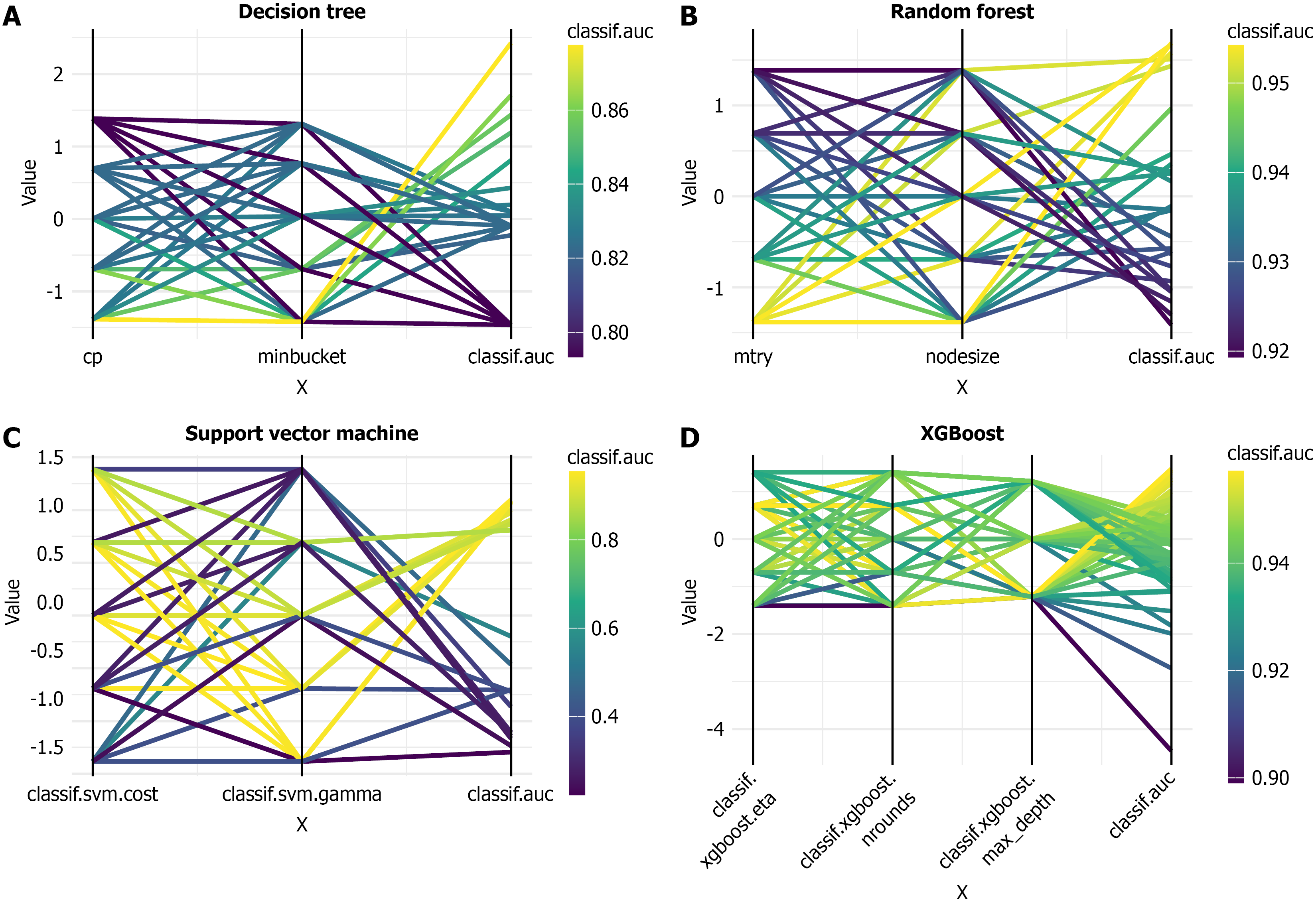
Figure 1 Visualization analysis of hyperparameter tuning results. A: Visualization diagram of decision tree hyperparameter tuning results; B: Graphical representation of random forest hyperparameter optimization; C: Support vector machine hyperparameter adjustment visualization; D: XGBoost hyperparameter adjustment diagram.

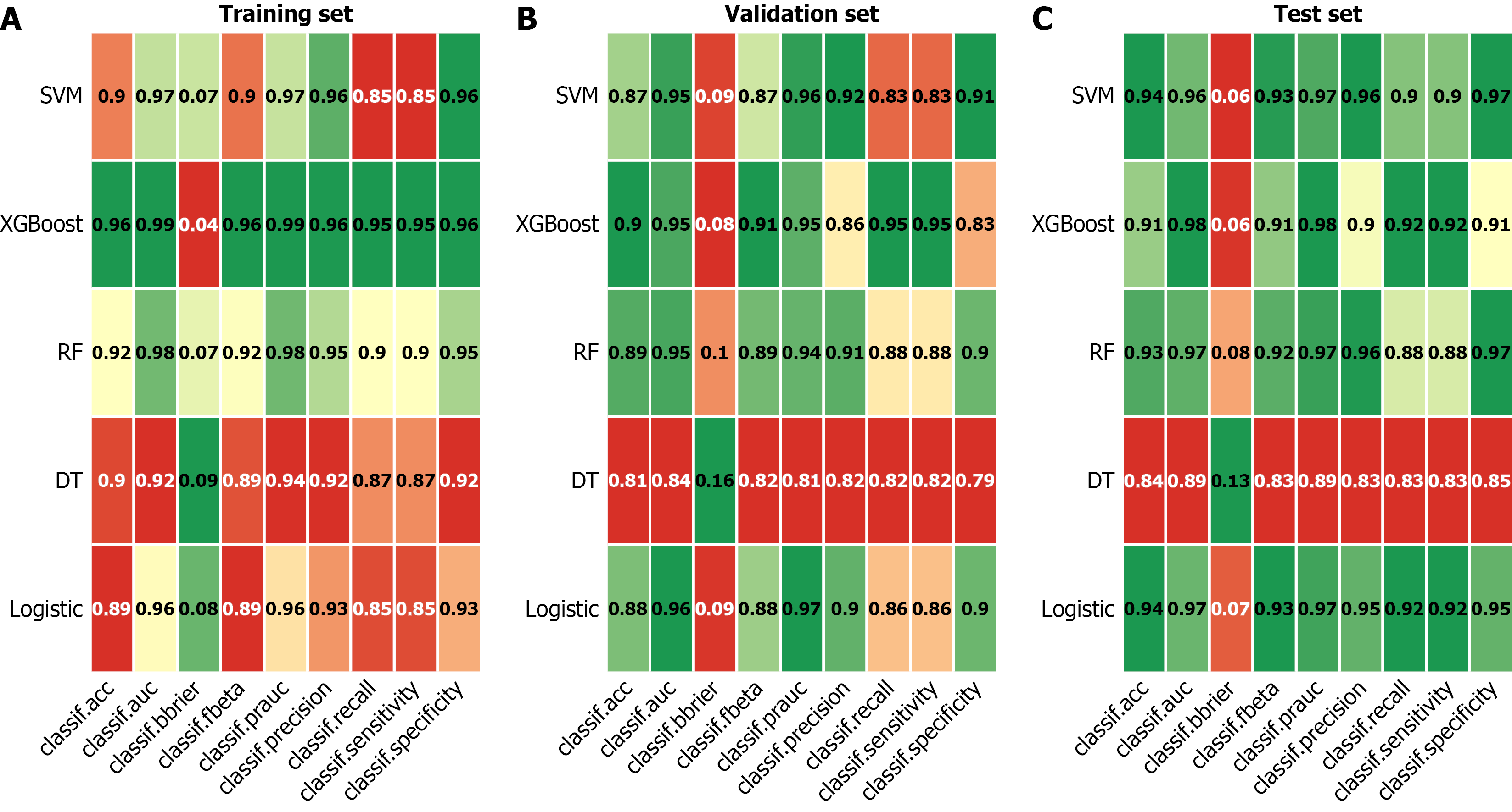
Figure 2 Heatmap visualization of classification models’ performance across training, validation, and test sets. A: Training set; B: Validation set; C: Test set. SVM: Support vector machine; RF: Random forest; DT: Decision tree.

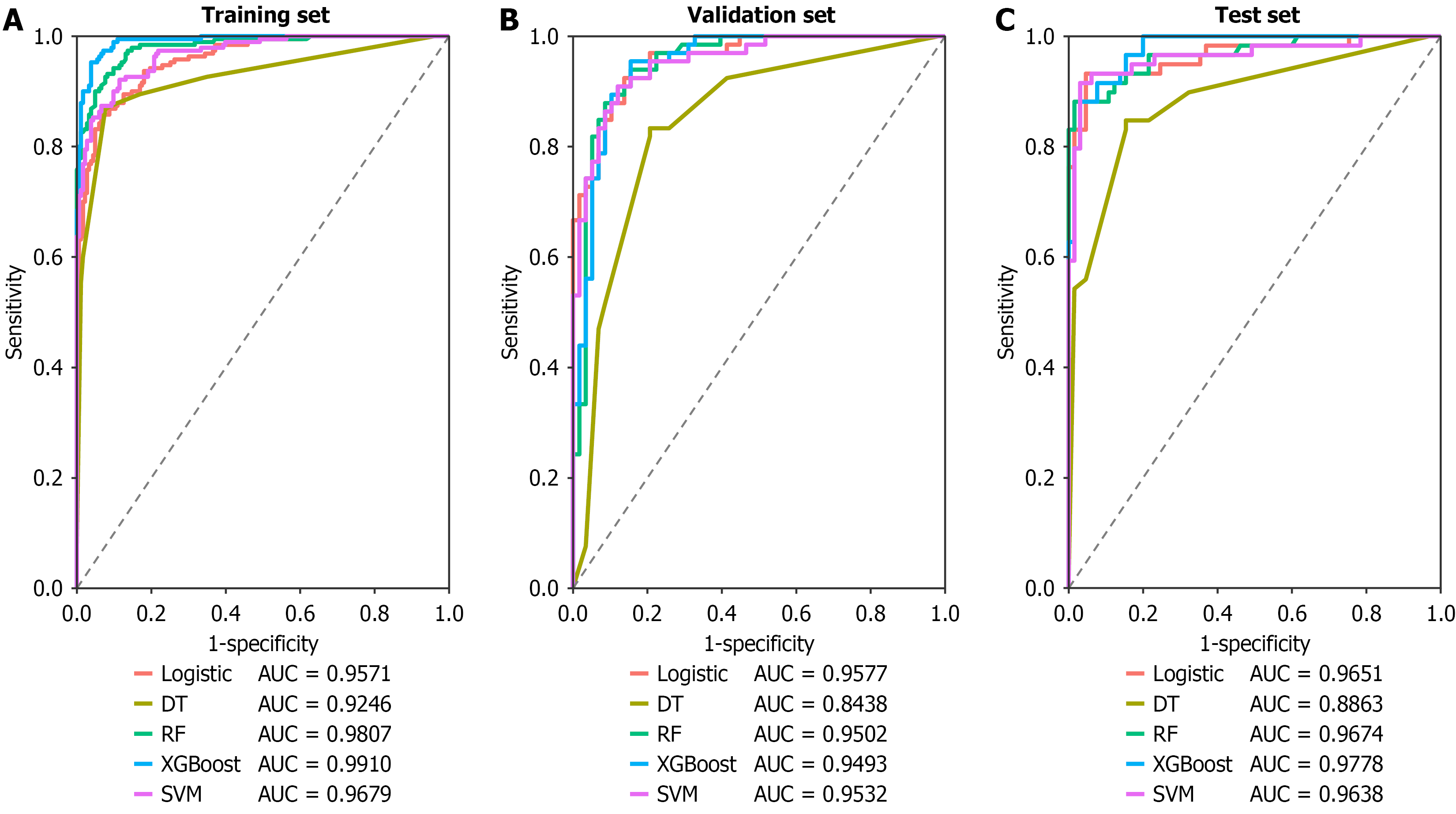
Figure 3 Receiver operating characteristic curves depicting model performance across different data partitions. A: Training dataset receiver operating characteristic (ROC) analysis; B: Validation dataset ROC analysis; C: Test dataset ROC analysis. AUC: Area under the curve; SVM: Support vector machine; RF: Random forest; DT: Decision tree.

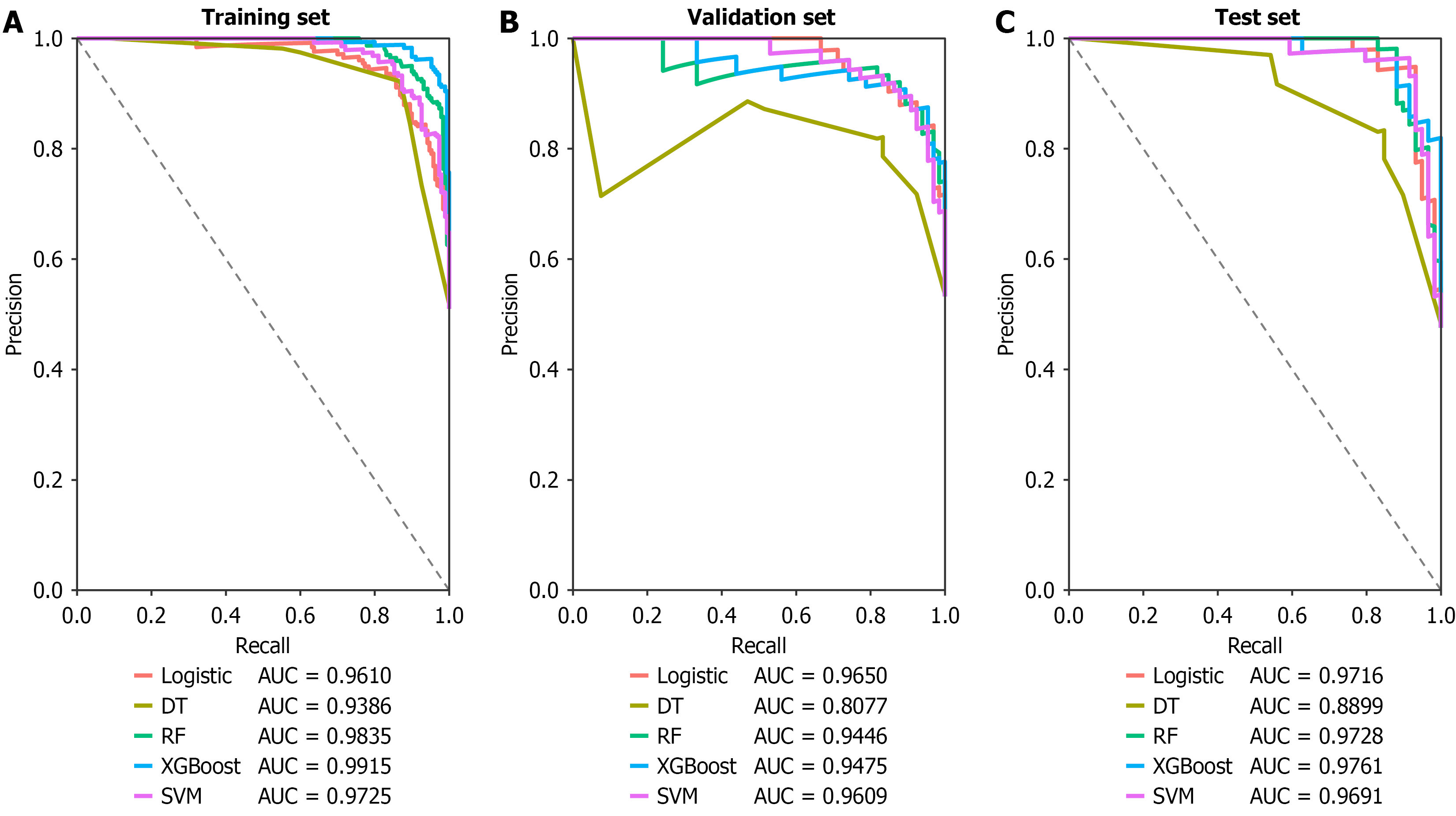
Figure 4 Precision-recall performance of the classifiers on multiple datasets. A: Training dataset precision-recall (PR) curve; B: Validation dataset PR curve; C: Test dataset PR curve. AUC: Area under the curve; SVM: Support vector machine; RF: Random forest; DT: Decision tree.

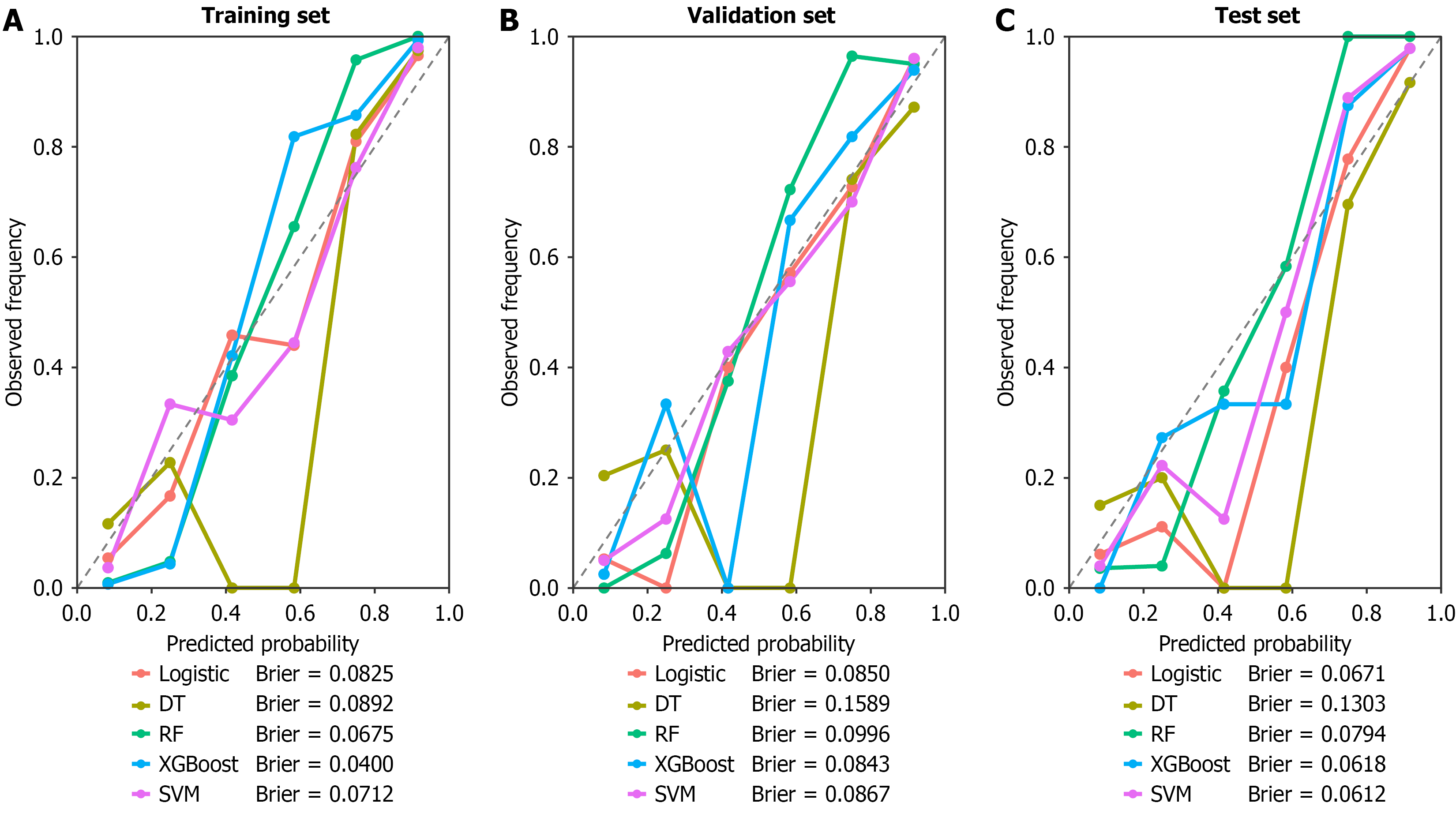
Figure 5 Model calibration plots for different data partitions. A: Calibration performance on training data; B: Validation data calibration results; C: Test set calibration analysis. SVM: Support vector machine; RF: Random forest; DT: Decision tree.

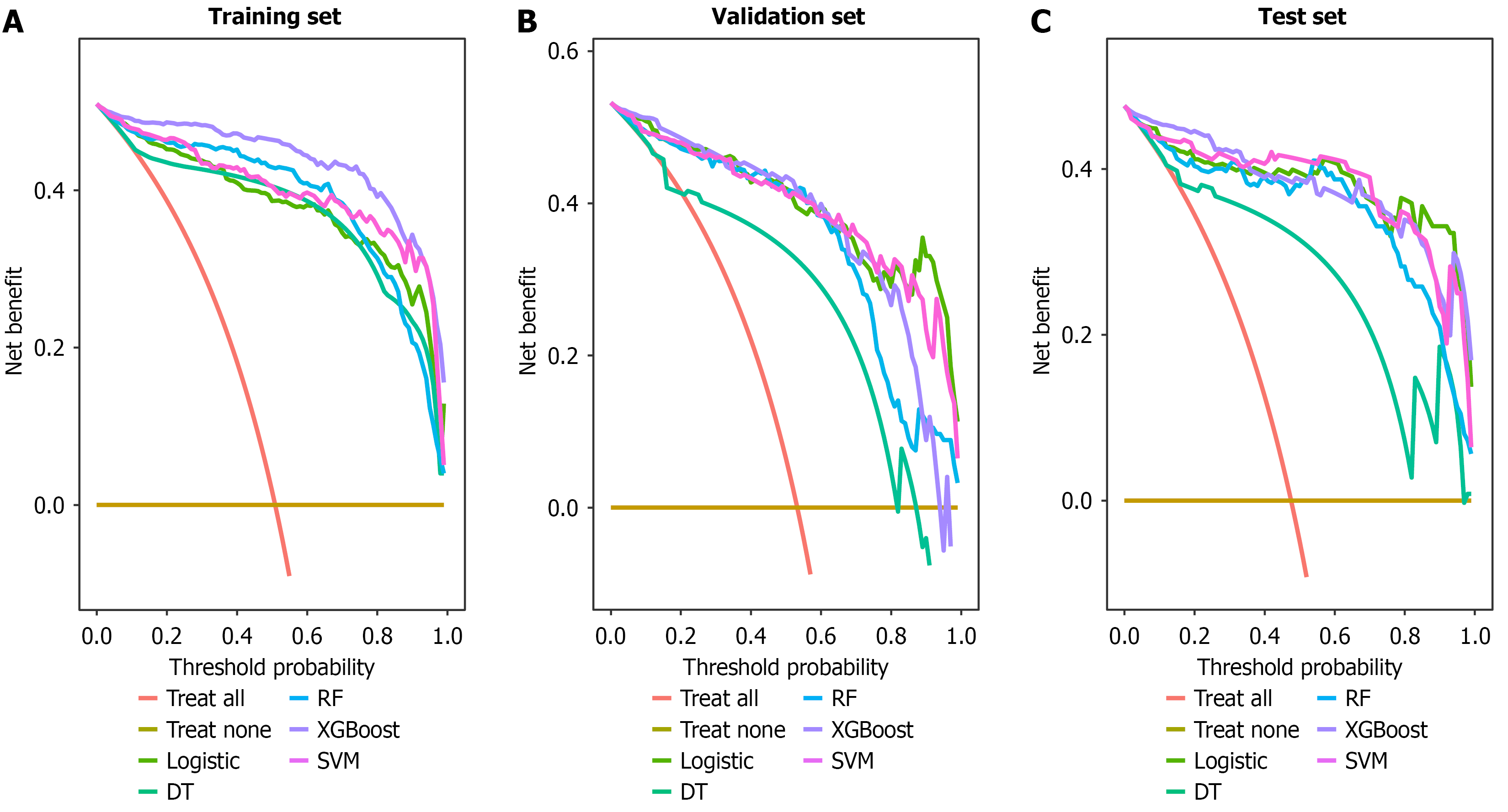
Figure 6 Decision curve analysis of different classifiers. A: Training set decision curve analysis (DCA); B: Validation set DCA; C: Test set DCA. SVM: Support vector machine; RF: Random forest; DT: Decision tree.

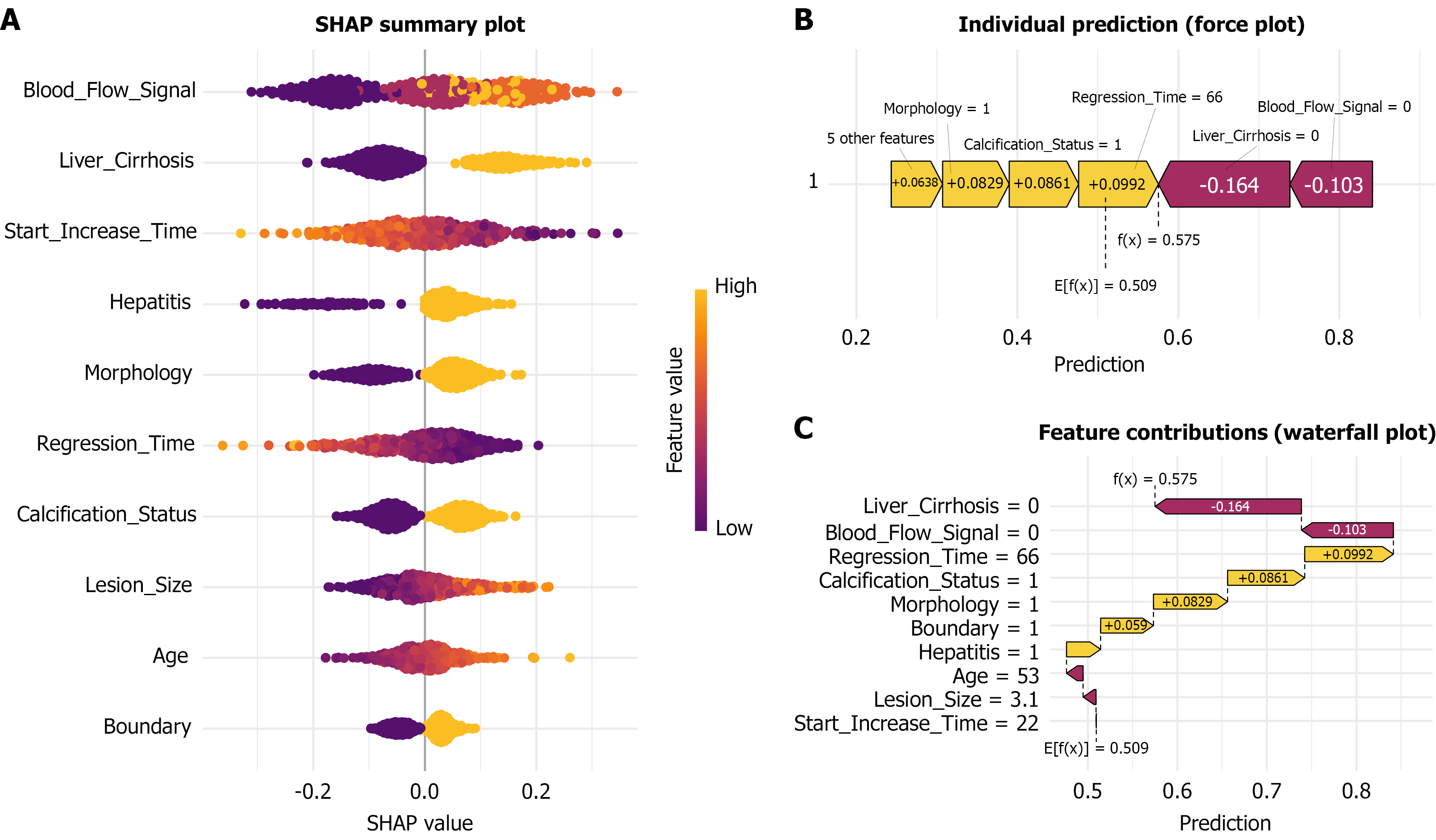
Figure 7 SHapley Additive exPlanations analysis and prediction examples. A: SHapley Additive exPlanations summary plot; B: Example of individual prediction; C: Detailed information presentation. SHAP: SHapley Additive exPlanations.

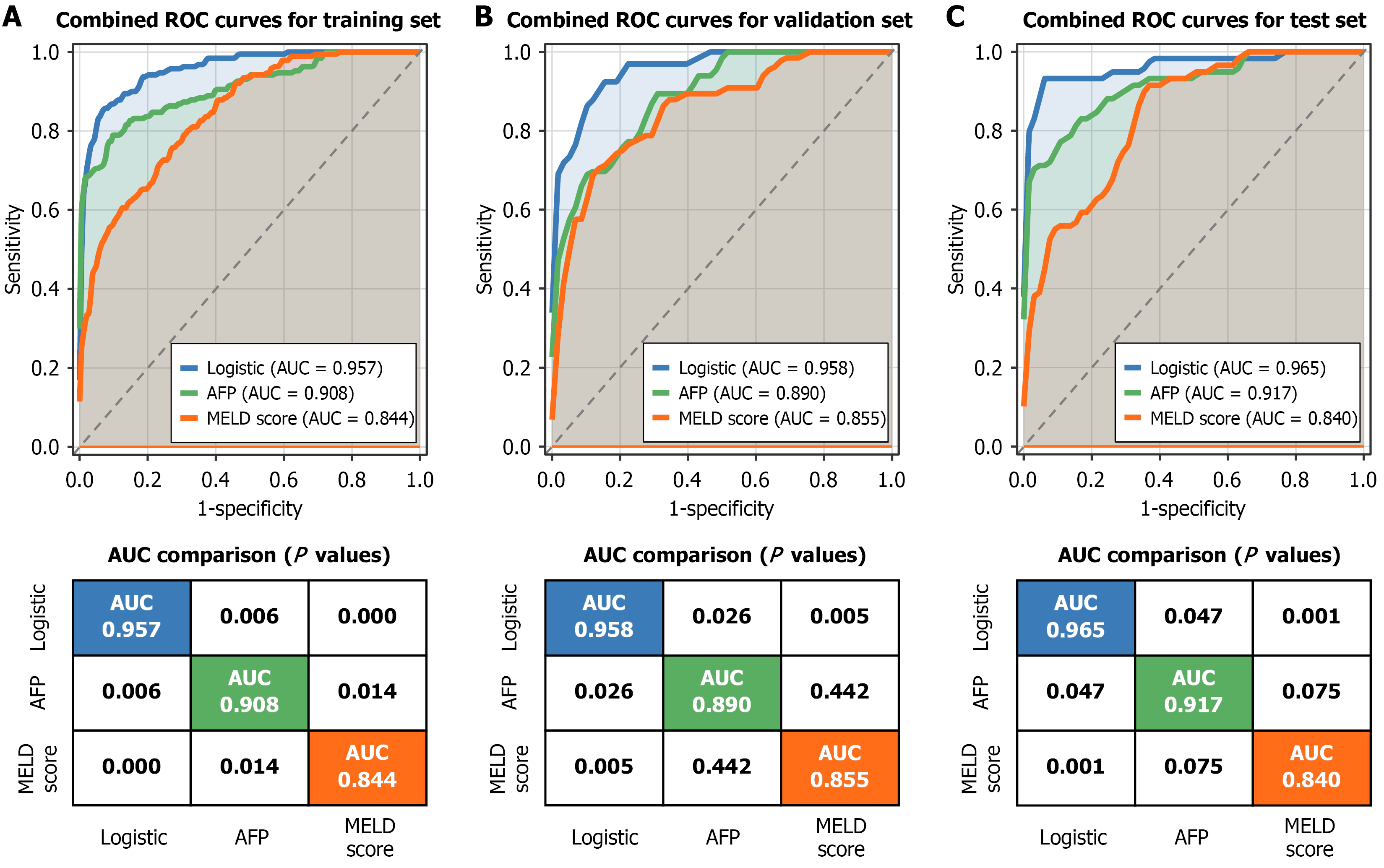
Figure 8 Comparative assessment of diagnostic performance between Logistic Regression model and conventional biomarkers using receiver operating characteristic analysis. A: Receiver operating characteristic (ROC) curve evaluation in the training cohort; B: Validation set ROC curve analysis; C: Test set ROC curve evaluation. ROC: Receiver operating characteristic; AUC: Area under the curve; AFP: Alpha-fetoprotein; MELD: Model for End-Stage Liver Disease.