Published online Oct 18, 2013. doi: 10.5312/wjo.v4.i4.267
Revised: August 21, 2013
Accepted: September 18, 2013
Published online: October 18, 2013
Processing time: 171 Days and 19.5 Hours
AIM: To determine if rabbit models can be used to quantify the mechanical behaviour involved in tibial stress fracture (TSF) development.
METHODS: Fresh rabbit tibiae were loaded under compression using a specifically-designed test apparatus. Weights were incrementally added up to a load of 30 kg and the mechanical behaviour of the tibia was analysed using tests for buckling, bone strain and hysteresis. Structural mechanics equations were subsequently employed to verify that the results were within the range of values predicted by theory. A finite element (FE) model was developed using cross-sectional computer tomography (CT) images scanned from one of the rabbit bones, and a static load of 6 kg (1.5 times the rabbit's body weight) was applied to represent running. The model was validated using the experimental strain gauge data, then geometric and elemental convergence tests were performed in order to find the minimum number of cross-sectional scans and elements respectively required for convergence. The analysis was then performed using both the model and the experimental results to investigate the mechanical behaviour of the rabbit tibia under compressive load and to examine crack initiation.
RESULTS: The experimental tests showed that under a compressive load of up to 12 kg, the rabbit tibia demonstrates linear behaviour with little hysteresis. Up to 30 kg, the bone does not fail by elastic buckling; however, there are low levels of tensile stress which predominately occur at and adjacent to the anterior border of the tibial midshaft: this suggests that fatigue failure occurs in these regions, since bone under cyclic loading initially fails in tension. The FE model predictions were consistent with both mechanics theory and the strain gauge results. The model was highly sensitive to small changes in the position of the applied load due to the high slenderness ratio of the rabbit’s tibia. The modelling technique used in the current study could have applications in the development of human FE models of bone, where, unlike rabbit tibia, the model would be relatively insensitive to very small changes in load position. However, the rabbit model itself is less beneficial as a tool to understand the mechanical behaviour of TSFs in humans due to the small size of the rabbit bone and the limitations of human-scale CT scanning equipment.
CONCLUSION: The current modelling technique could be used to develop human FE models. However, the rabbit model itself has significant limitations in understanding human TSF mechanics.
Core tip: In the current study, experimental and finite element (FE) analysis demonstrated that under compression, the rabbit tibia exhibits linear behaviour. The stresses in the rabbit tibia are sensitive to small changes in load position due to its high slenderness ratio. Low tensile stresses occur at the anterior border of the midshaft, suggesting that this region fails in fatigue, as bone under cyclic loading initially fails in tension. The current modelling technique could be used to develop human FE models.
- Citation: Franklyn M, Field B. Experimental and finite element analysis of tibial stress fractures using a rabbit model. World J Orthop 2013; 4(4): 267-278
- URL: https://www.wjgnet.com/2218-5836/full/v4/i4/267.htm
- DOI: https://dx.doi.org/10.5312/wjo.v4.i4.267
Core tip: In the current study, experimental and finite element (FE) analysis demonstrated that under compression, the rabbit tibia exhibits linear behaviour. The stresses in the rabbit tibia are sensitive to small changes in load position due to its high slenderness ratio. Low tensile stresses occur at the anterior border of the midshaft, suggesting that this region fails in fatigue, as bone under cyclic loading initially fails in tension. The current modelling technique could be used to develop human FE models.
Stress fractures are fatigue fractures which occur in normal bone subjected to atypical cyclic loading. This altered stress state results in microcracks in the cortical bone tissue due to bone failure. Most commonly sustained in the tibia, stress fractures are debilitating injuries, often requiring weeks to months of rest and rehabilitation. Despite various interventions introduced in order to mitigate the risk of stress fractures, athletes[1-3] and military recruits[4,5] continue to be susceptible to these injuries due to their intense training regimes.
In previous research, tibial stress fractures (TSFs) have been analysed using rabbit bones as they are relatively inexpensive and easy to acquire. However, the rabbit and human tibia differ anatomically, with one of the primary distinctions being the distal articulation of the tibiofibula complex: in the human it is near the ankle joint whereas in the rabbit it is at the tibial midshaft.
In some earlier research where TSFs were produced in rabbit tibiae, 20 rabbits were trained to run and jump in response to electrical stimulation so the applied loads to the rabbit bones were equivalent to a human performing impact exercise[6]. By sacrificing the rabbits at various stages during the experiment, the radiographic and histological changes in the bone over a 60-d period could be analysed. Although this study provided invaluable data on the development of TSFs, the exact loads to the tibia were unknown as only the electrical stimulation could be controlled, and not the loading.
In order to overcome the above limitation, another research group later used a specifically-designed apparatus which could apply compressive cyclic loads to rabbit hind limbs[7]. The device was subsequently used to load the tibia of 31 rabbits by approximately 1.5 times their body weight on one limb, using the other unloaded side as a control. Scintigraphically-confirmed TSFs were successfully produced in 68% of the rabbits within six weeks of the loading regime. The same researchers later developed a finite element (FE) model of a rabbit’s tibia[8,9]. However, there were significant limitations with both their experimental and modelling approach. For example, the rabbits were not under anaesthetic; hence, in addition to the applied compression, bending forces could be produced by involuntary muscle contraction. The results of the FE model were also anomalous.
In a more recent study, rabbit tibiae were fatigue tested under three-point bending with the aim of determining fatigue resistance due to age and sex differences[10].The authors found there were differences in fatigue behaviour due to age but not sex; fatigue resistance increased with both greater skeletal maturity and increased bone mineral density. However, it is not possible to determine from this research where rabbit tibia may fail in-vivo due to normal physiological loading as three-point loading can only be used to evaluate fatigue in a localised area of the tibial mid-diaphysis, but not the fatigue behaviour of the remaining bone.
Using a combination of experimental analysis and FE modelling, the aim of the current research was to quantify the mechanical behaviour of the rabbit tibia and to determine the stresses in the bone when subjected to typical applied compressive loads representing the rabbit running. A secondary aim was to design a method which could be later used to develop FE models of human bone.
Tibiae were harvested from rabbits obtained from the Monash University Department of Physiology in accordance with the Australian Code of Practise for the Use of Animals for Scientific Purposes (7th Edition, 2004). Experimental work was initially performed to determine the mechanical behaviour of the rabbit’s tibia; one of these tests was also used for FE model validation. The experiments were performed first, thus enabling fresh wet specimens to be tested before the bone was imaged by computed tomography (CT) for the FE model geometry. Mechanical compression and beam theory analysis were also used to verify the results.
Rabbit sample preparation: One English Cross-Breed and two New Zealand White Rabbits (NZWRs) were sacrificed with an overdose of pentobarbitone sodium (300 mg/kg) intravenously and the hind limbs were dissected from the rabbits with the musculature and tissues still intact. The limbs were separated, wrapped in gauze bathed in physiological saline to keep them moist, then frozen for later use. Prior to each experiment, the right limb (for consistency) was removed from frozen storage and saturated in tepid saline to thaw the tissues while keeping the tibia moist. After thawing, the limb was removed from the water bath and the tibia/fibula complex was dissected from the remaining tissue.
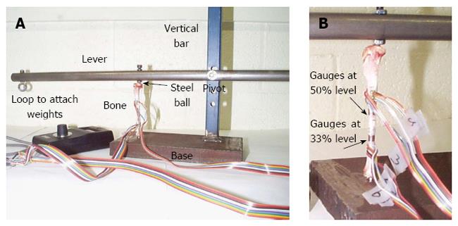
Rabbit tibial experiments: A purpose-built rig consisting of a vertical bar attached to a base and a pivoting lever on the bar was assembled (Figure 1A). Calibrated weights were applied to the loop at one end of the lever, thus loading the bone, which was located one third the distance between the pivot and the weight. The tibia was retained by a steel ball at each end; this enabled the bone to remain fixed during the test, and more importantly, facilitated bone loading through a concentrated rather than a distributed load, which could then be easily replicated in the FE model. Three tests were conducted: (1) a buckling test, to quantify bone deflection and linear behaviour under axial load; (2) a strain gauge test, to obtain stresses for FE model validation; and (3) a hysteresis test, which in addition to measuring hysteresis, was used to verify that the strain gauges had adhered properly to the bone. The English Cross-Breed Rabbit tibia was used in the first experiment, while NZWR tibiae were used in the subsequent experiments. After the strain gauge test, the tibia was then CT scanned in order to obtain the geometry for the FE model.
In the first experiment, weights were incrementally added to the loop on the pivoting rod to compress the bone and a dial gauge was used to measure the deflection of the bone in the anteroposterior (AP) direction at the midshaft for each successive increase in load. In the second and third experiments, the strain gauges were bonded to the tibia in predetermined locations using M-Bond 200 cement. Although the positions chosen were somewhat arbitrary as the aim was to validate the FE model in different locations, the magnitude of the stresses in the areas where TSFs[2,4,8,11,12] and Medial Tibial Stress Syndrome[2,13] are sustained were of interest; hence the gauges were attached to those sites.
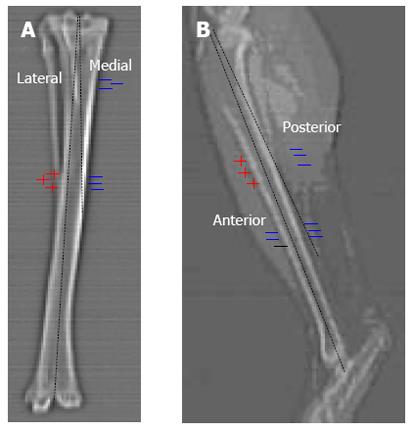
As shown in Figures 1B and 2, four strain gauges (anterior, posterior, medial and lateral) were attached at the junction of the mid and distal thirds of the tibia (33% of the tibial length from the distal end of the tibia) and four strain gauges were attached in the centre of the midshaft (50% of the tibial length from the distal of the end of the tibia), where the tibial length was defined to be the distance from the medial malleolus to the medial joint line. A hand-held strain gauge reader was used to record measurements from the gauges.
Geometry: Using a Hitachi W1000GR scanner (Hitachi Medical Corporation, Tokyo, Japan), one scout film and 71 consecutive tibial cross-sectional CT images 1.55 mm apart were scanned; this was the maximum number of cross-sections which could be imaged due to the small size of the rabbit bone. These images were used to create a base, or reference, model. The cross-sections were automatically aligned by the CT scanner using the origin of each image, which was located at the top left corner. The images were digitised from DICOM format to TIFF format using eFilm (Merge Healthcare) software. In order to ensure the load position in the computer model was the same as the load position in the experiments, a point at each end of the bone was marked using a scalpel. These points, which approximately corresponded to the physiological load positions, could be later visualised on the CT scans.
The University of Texas Health Science Center at San Antonio ImageTool for Windows (Version 2.0, San Antonio) software was used to display the images and to generate data points for the geometry. To eliminate user variability, one person performed all measurements. To find the optimum number of data points required around a cross-section, convergence tests were performed using a Fortran program, where a number of cross-sectional properties were computed while varying the number of perimeter points. More details on these tests can be found in previous publications[2,14]. The third co-ordinate was based on the CT scan position along the longitudinal axis. As only the cortical bone was of interest, any regions of indistinct bone were not included in the data acquisition.
To create the solid model, two FE packages, Abaqus CAE (Version 5.0) and Hypermesh 3D (Altair, Versions 6.2 and 7.0), were used in conjunction with a specifically-written Python script. The Python code was executed in Abaqus, which then automatically generated a command file and used the data points to produce a series of cross-sectional splines by cubic spline interpolation. The command file was subsequently executed within Hypermesh to create the wireframe model from the spline data. The solid model geometry and the remainder of the pre-processing were performed using Hypermesh.
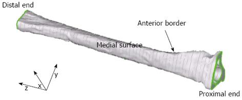
Six slices were truncated from each end of the 71 CT images as the complex geometry at each end is laborious to model and not of interest in the current study. Thus, the final base model was 90 mm in length and was comprised of 59 equally-spaced CT slices 1.55 mm apart. The model was meshed with 28248 parabolic 10-nodded tetrahedral elements 0.77 mm apart. The tetrahedral element length was the smallest distance which could be meshed without the model developing numerical instabilities, for example, instabilities which resulted from the average distance between adjacent nodes falling below the computational accuracy of the program. The final base model (Figure 3) was used as a reference to which other, less detailed, models could be compared.
Material properties: The material properties of rabbit bone available in the literature are limited. However, as the experimental results (presented later) demonstrated, linear elastic isotropic material properties could be presumed for loads up to 12.5 kg; hence, this assumption was used in the FE model. The value used for the Young’s Modulus (E) was the mean of the values from the rabbit femoral and humeral bone midshafts for wet cortical bone (since no Young’s Modulus was available for the rabbit tibia), thus E = 10950 MPa. A Poisson’s ratio of μ = 0.3 was used, which is the value of μ for both the rabbit femoral and humeral bone[15].
Boundary conditions: Using the Image Tool software, the scalpel marks at each end of the bone were identified on the CT scans and the 3D Cartesian co-ordinates were determined. With the neutral axis as a reference, the co-responding co-ordinates were found at the cross-sectional level where the model had been truncated (recalling that six CT scans were truncated at each end). A nodal point and a series of rigid beam elements were created at each end of the model in order to transfer load, with the number of beam elements controlled by the element density. A static axial load of 60 N, which represents approximately 1.5 times the body weight of the rabbit (i.e., a typical load representing the rabbit running), was applied to each end of the model. For quasi-static loading such as running, which can be represented as a step-function and occurs over a fraction of a second, static loading is appropriate[16]. This is consistent with FE models in the literature where, for example, femoral fractures from falls in the elderly have been evaluated using static FE analysis[17,18]. Conversely, impulse loads which are dynamic and occur over a period of milliseconds, such as ballistic and automatic impacts, require dynamic FE models.
FE model analyses: The models were executed using the OptiStruct solver, and then the post-processing was performed using Hypermesh (Altair, Versions 6.2 and 7.0). In order to validate the model, the von Mises stresses were plotted for the base rabbit model and then compared to the experimental strain gauge results at eight locations. Due to the high mesh density, there were many nodes on the model corresponding to a particular strain gauge location on the rabbit; hence, the stresses at several nodes in the relevant region of the model were measured and the results averaged. A sensitivity analysis was then conducted by moving the axial load on the full model to four other positions so the change in stresses due to distance from the centroid could be investigated.
Geometric and elemental convergence tests were performed in order to establish the minimum number of cross-sections and elements respectively required in a reduced FE model to produce similar stresses to the base rabbit model with the 59 cross-sections. Geometric convergence tests were conducted by reducing the number of cross-sections while the tetrahedral element length was kept constant. After the optimal number of cross-sections was ascertained, the elemental convergence tests were performed using a constant number of cross-sections but reducing the number of elements.
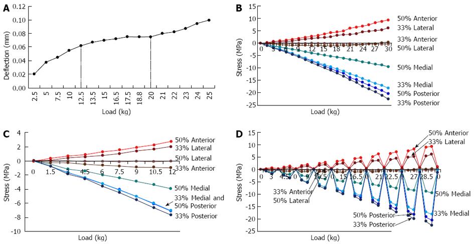
Elastic buckling test: For lower axial loading levels, the rabbit tibia demonstrated linear behaviour, particularly for loads less than 12.5 kg (Figure 4A), or 122.5 N (throughout the paper, mass has been used as a convenient representation of force). There was non-linear behaviour at higher loads, although the non-linear region (> 12.5 kg) also demonstrated linear behaviour (20-25 kg). At a maximum load of 25 kg, the deflection was 0.1 mm anteriorly in the AP direction at the centre of the anterior midshaft (measured by the dial gauge). Using the CT images, the bone length was measured to be 100 mm and the width in the AP direction at the midshaft was 7.5 mm. Hence, the deflection of the bone was 1.33% of the AP width and 0.1% of the tibial length. These results demonstrated that not only did the bone not buckle, but the rabbit’s tibia is not particularly flexible under load.
Using mechanics theory, the expected buckling load was calculated for a straight, uniform column having the same midshaft AP dimension as the rabbit’s bone. The slenderness ratio was 59 (Le/p ≈ 100 mm/1.7 mm), where Le is the equivalent length of the column and p is the radius of gyration. Using the Fortran program, the value of p was numerically computed from the CT scan at the centre of the tibial midshaft. A slenderness ratio of 59 (i.e., a slenderness ratio > 10) represents a long slender column. The critical loading limit, Pcr :
Pcr = ≈ 105 kg
where E, Imin and Le are the Young’s Modulus (kg/mm2), the minimum second moment of area (mm4) and the equivalent length (mm2) respectively[19]; in an irregular bone such as the rabbit tibia, Imin is along the axis where I is minimised, although in the cylinder here I is the same in all directions. Since the rabbit tibia is bent (the line of loading does not pass through the centroid of the mid-point cross-section), it would be expected to buckle at less than 105 kg, but highly unlikely to buckle at 25 kg. This is consistent with the experimental results.
If the rabbit tibia was quite flexible, then the compressive load acting may cause the neutral axis (i.e., the axis through the centroids of all cross-sections) to shift further away from the line of action of the compressive load. This increase in offset distance has the potential to produce additional tension in the bone due to the creation of bending stresses. The experiment demonstrated that bone was not particularly flexible; hence, under a compressive axial load, the stress in the bone is predominately compressive. Any tensile stress would be produced on the anterior border due to the forward curvature of the bone.
This is discussed further under the section Mechanical theory predictions.
Strain gauge test: Strains were measured from eight gauge locations in increasing 1.5 kg loads, then converted to stress using the Young’s Modulus (defined earlier) for rabbit bone (Figure 4B). Two gauges, the 33% level anterior and the 50% level lateral, were unstable and remained close to zero as it was difficult to keep the device fixed at the precise loading point for very small loads. Examination of the output strains at near-zero loads demonstrated that the strains were sensitive to small changes in the point of load application. At higher loads, the strains were stable due to the compression applied through the loading device onto the bone.
The stress-strain graphs are slightly non-linear (Figure 4C), consisting of two linear curves (approximately 0-15 kg and 18-30 kg) joined by a non-linear segment (approximately 15-18 kg). Thus, linearity for loads up to approximately 12 kg can be assumed, and in particular, linearity for loads simulating a rabbit running (about 6 kg) can be used.
Hysteresis test: Although the rabbit tibia displayed some hysteresis (Figure 4D), it was not extensive, but gradually increased with increasing load. For example, for a load of 30 kg, the maximum compressive and tensile stresses were -22.6 MPa and +9.4 MPa respectively, representing a corresponding hysteresis of approximately -1.1 MPa and +1.0 MPa (i.e., 5% hysteresis in compression and 10.5% hysteresis in tension). At a load of 6 kg, the hysteresis was approximately 0.5% (-0.12 MPa) in compression and 2% (+0.19 MPa) in tension. Hence, there was no significant hysteresis. These results demonstrated that (1) the gauges had adhered to the bone and (2) the bone demonstrates elastic behaviour for loads up to 30 kg. When considered in conjunction with the results from Figure 4A, it can be concluded that for loads up to 12.5 kg, rabbit bone shows linear elastic behaviour, while for loads between 12.5 kg and 30 kg, rabbit bone is elastic but shows some non-linearity. Thus, for loading which represents a rabbit running (6 kg), linear elastic behaviour can be assumed.
The minimum offset distance required to produce tension on the opposite side of a beam when a compressive force is applied can be calculated from mechanics theory. A net tension can occur in the section when the tensile bending stress caused by the offset is greater than the magnitude of the stress caused by the compressive load.
Assuming a hollow cylinder where r2 > r1, the bending moment stress (σBM ) can be calculated by:
σBM = my/ I
where m is the bending moment, y is the distance from the centroid to the point the stress is being calculated (equal to the maximum radius of the cylinder) and I is the second moment of area.
However, m = Fx and I =π/4[(r24 - r14)], where F is the compressive force, x is the offset distance of the load from the centroidal axis and r2 and r1 are the outer and inner radii mentioned above. Hence, substitution of the equations for m and I into the bending moment equation:
σBM = 4Fxy/π(r24 - r14)
The compressive stress (σC ) can be calculated by:
σC = F/A where F is the applied force and A is the cross-sectional area. The area can be described in terms of the inner (r1) and outer (r2) radii of the section:
A = π/4[(2r2)2 - (2r1)2]
Substitution of the area equation into the compressive stress equation:
σC = 4F/π[(2r2)2 - (2r1)2]
Hence σC = 4F/π(4r22 - 4r12)
σC = F/π(r22 - r12)
If σBM > σC , then tension can be produced on the opposite side of the beam.
This is satisfied when:
4Fxy/π(r24 - r14)> F/π(r22 - r12)
Simplifying 4Fxy/(r24 - r14) > F/(r22 - r12)
Solving for x, the distance between the centroid and the load position:
x > (r24 - r14)/ 4y(r22 - r12) but y = r2 (maximum)
Hence: x > (r24 - r14)/ 4r2(r22 - r12)
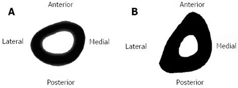
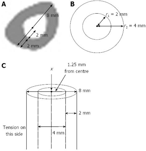
If the dimensions of the rabbit tibia at the centre of the midshaft are 8 mm in width, where 4 mm is the medullary region and 2 mm each end is comprised of cortical bone (approximate measurements from CT images, as shown in Figure 5A, and shown on a beam cross-section in Figure 5B), then the equation is satisfied when:
x > (44 - 24)/ 4(4)(16 - 4) > 240/ 192 mm
Hence x > 1.25 mm
Thus, a load applied at one end of the bone would only need to move 1.25 mm away from the centroid (less than half the medullary width) in the x - y plane to produce tension in the midshaft on the opposite side of the bone. This is demonstrated in Figure 5C. Tension can also arise from a slight curvature of the tibia (i.e., when it is bent by 1.25 mm or more), such as via the natural curvature which already exists in the bone (Figure 6).
Convergence tests on the FE model: The base model, which was used as a reference, was 90 mm in length and contained 59 equally-spaced CT slices 1.55 mm apart (Figure 3, shown earlier). As mentioned previously, the mesh was comprised of 28248 parabolic 10-nodded tetrahedral elements 0.77 mm apart. The von Mises stresses were computed since sites of high stress intensity were of interest because these would indicate where local yielding may occur and hence initiate microfractures.
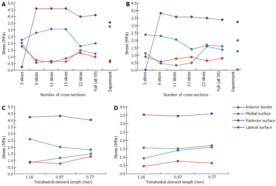
The geometric convergence test results are shown in Figure 7A and B (at the mid-distal junction and midshaft respectively). At the mid-distal junction, the results have clearly converged when the model has 22 cross-sections, as demonstrated by the fluctuating stresses for the results of the last three cross-sections (i.e., the 13, 22 and 59 cross-sections). Similarly, at the midshaft, the stresses have converged by 22 cross-sections for all regions except the posterior surface, which is on the point of convergence. Hence, a model with 22 cross-sections is sufficient for the analysis, i.e., will give comparable stresses to the full model with 59 cross-sections.
The mesh convergence test results demonstrate that all regions have converged or almost converged (Figure 7C and D). When the model was meshed with elements of tetrahedral element lengths of 0.4 mm, and then 0.58 mm, the simulation aborted due to numerical instabilities as adjacent nodes were too close. Hence, a tetrahedral element length of 0.77 mm was the finest mesh which could be achieved in the rabbit model due to the small dimensions of the bone (this would not be an issue in a larger structure, such as a model of the human tibia). A comparison of the convergence data shows that the variation in stress is considerably greater for the geometric convergence test than the mesh convergence test, indicating that it is more critical to have a greater number of cross-sections than a more refined mesh in the rabbit model.
Beam theory and experimental results: Results from the beam theory predictions and the strain gauge experiments were plotted on the same graphs for comparison (Figure 8). For the beam theory analysis, an axial compressive load between the two condyles of the tibia was used in conjunction with standard engineering equations for a hollow non-circular cylinder.
Under an axial load of 6 kg, the predicted stresses were all compressive at the mid-distal tibial junction. At the midshaft, the stresses were all compressive, except at and adjacent to the anterior border. The experimental results were reasonably consistent with the calculated values, excluding the lateral gauge, where there was some disparity.
FE model results and sensitivity tests: The von Mises stress contours from the FE model were plotted in conjunction with the stress moduli (since von Mises is a positive entity) from the beam theory and experimental results at the mid-distal junction and the midshaft (Figure 9A). At the mid-distal junction, there was good agreement between the FE model, the beam theory results and the experimental values for the posterior and lateral surfaces; however, at the medial surface and anterior border, there was some disparity between the FE model and the other results. The FE results for the midshaft were fairly close to both beam theory and experimental results in all four locations.
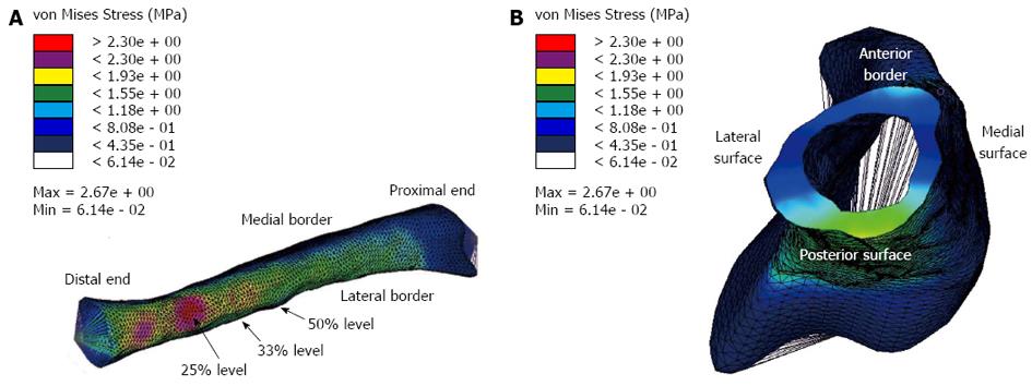
Figure 9A demonstrates a colour contour plot of the von Mises stress distribution in the rabbit model. There were high stresses along a large region of the posterior surface of the model; this was reflected in the experimental results where the highest (compressive) stresses at the 33% and 50% levels were on the posterior strain gauge (shown earlier in Figure 8). Figure 9B demonstrates a view of the model truncated at the 50% level; these stresses were consistent with the strain gauge results shown in earlier in Figure 8B (note that exact numbers cannot be compared as the gauges in the experiments cover a region, where the stresses are then averaged). The model also showed that highest stresses were not at the 33% and 50% (where the strain gauges were located in the experiments), but around the 23% level of the tibia (Figure 9A). In order to explore this further, the principal moments and cross-sectional area for the rabbit cross-sections were numerically calculated using the Fortran program and plotted (Figure 10).
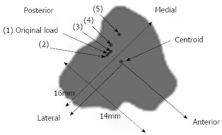
The illustration of the sensitivity test, where the applied load was moved to a number of positions near the original load and the centroid of the cross-section, is shown in Figure 11. The results of the sensitivity test and comparison with the beam theory and experimental results are shown in Figure 12.
The results demonstrated that it was probable that the load position was in fact posteromedial to Load 1 (i.e., posterior to Load 2, Figure 11), which is 1-2 pixels from the original load, based on measurements made using the imaging software. Moving the load position one pixel (i.e., about 0.4 mm) resulted in a significant change in the stress output, particularly in the anterior and medial positions (up to 27% on the anterior border); hence, the rabbit FE model stresses are highly sensitive to load position, which is consistent with the large slenderness ratio of the rabbit tibia.
As shown by predictions using engineering mechanics, experimental data and FE analysis, a compressive point load between the two condyles of the rabbit tibia will predominately result in compressive stresses throughout the bone. The highest compressive stress is on the posterior surface, around the 24%-28% level of the bone, which also corresponds to the regions which have the lowest cross-sectional areas and principal moments. Tension is produced predominately on the anterior border of the midshaft, but also on the anterolateral region at the midshaft and distal thirds. The magnitude of tension is not high, and since the rabbit bone is not particularly flexible under load and does not buckle, this tension is likely to remain low. Bone generally fails in tension from static loading[20], while under cyclic loading, cortical bone fails in tension before compressive failure later occurs after repeated loading[21,22]. Hence, the results suggest that TSFs in the rabbit model are produced in the anterior midshaft by low levels of tensile stress i.e., the region of least compressive stress.
In the current study, the stresses in the rabbit bone primarily demonstrated linear behaviour (for up to three times the rabbit’s body weight) with little hysteresis. Previous work has shown that stress-strain curves of a number of different animal bones are similar to those of human bones, with the only difference being the Young’s modulus[15]. Hence, linearity can be assumed for the human tibia for static loading up to three times body weight. The FE model of the rabbit tibia also demonstrated that the stresses were exceptionally sensitive to small changes in loading position (to the level of one pixel, or 0.4 mm), which is not surprising, because the rabbit tibia has a large slenderness ratio. This differs to the human tibia, which is considerably wider relative to its length; hence, the same sensitivity to small changes in load position would not be expected in a human tibia.
In previous studies, rabbit models have been used to study TSFs. In some earlier research by Li and colleagues[6], rabbits were trained to run and jump when subjected to electrical stimuli. The histological analysis from these experiments demonstrated that cracks developed on the cement lines of the Haversian systems, most frequently in the midshaft of the tibia (16 tibiae), followed by the distal third (3 tibiae) and lastly the upper third (1 tibia). These cracks predominately developed on the anterior and medial aspects of the tibia. Fracture lines were then formed by convergence of adjacent cracks from the Haversian systems. This rabbit experiment provided in-vivo verification of the early cortical bone specimen tests in the literature, where it was found that tensile failure occurs first under cyclic loading, and this tensile failure resulted in osteon debonding at the cement lines[21,22]. Li et al[6] did not specify which types of cracks (longitudinal, transverse or oblique) occurred in the various locations of the tibiae. However, they did observe that most cracks occurred in the anterior and medial aspects of the midshaft, which was consistent with other research to date on tensile stresses and tensile failure at this site. The main limitation with their study was that the exact magnitude of loading to the bone was unknown and could not be controlled.
In a subsequent study by Burr and colleagues, this limitation was overcome by loading rabbits using a specifically designed apparatus which could apply compressive cyclic loads, where the magnitude was known and could be controlled, to the hindlimbs of 31 rabbits[7].TSFs were successfully produced in 68% of the rabbits within six weeks of loading and were verified by scintigraphy. Of these TSFs, 89% were in the midshaft (implying that 11% were distal) and 74% were anteromedial, although it was not clear how many of the midshaft TSFs were anteromedial. The authors later stated that the rabbit model frequently shows TSFs distally[23], although the 89% in the midshaft was not mentioned, suggesting that it is, in fact, difficult to determine the exact location of TSFs in the rabbit. This is not surprising, as scintigraphy only shows a region of increased radionuclide uptake and the exact location would be difficult to visualise in a small bone such as the rabbit tibia. Although the study by Burr and colleagues[7] demonstrated that TSFs could be produced using a controlled load, the main limitation was that the rabbits were not under anesthetic during loading; hence their muscles could involuntary contract. Hence, the loading applied to the tibia was not purely compressive, as the involuntary muscle contractions apply other loads to the bone such as bending (which is then accentuated by the natural bend in the tibia), resulting in tensile stresses on the anterior border of the tibia. Furthermore, if the knee of the rabbit was flexed significantly in the experiment, the load line may be outside the cross-sectional area of the bone, which would produce further tension on the anterior side of the bone.
Using the Patran FE package (MSC Software), the same researchers who designed the controlled loading apparatus (discussed above) later developed a FE model of the rabbit’s tibia where compressive loading only was applied[8,9]; the model was based on some earlier work by the same researchers[24]. However, there were a number of discrepancies with their FE model. For example, the model did not have any loads from the musculature applied other than compression, yet, as mentioned above, it is probable that the tibia was subjected to other loads, such as bending, in the rabbit experiments. More significantly, the results of the FE model showed that high compressive stresses occurred on the anterior border of the tibia, yet from clinical research and knowledge of fracture types at this site, TSFs on the anterior border are a result of tensile failure due to tensile or bending forces[13,25,26]. In order to produce large compressive stresses on the anterior border (and tensile stress on the posterior surface), the load line would need to be significantly forward of the centroid, particularly as the tibia is bent anteriorly and the rabbit leg is partially flexed (Figure 12). However, this is not consistent with the load position in the experiments, as the load was applied to the rabbit's heel; hence the load line would be posterior to the centroid.
While supporting body weight, the tibia is under compression; however, the tibia experiences both compressive and tensile stresses. Tension can arise from elastic buckling, from compressive loading, and from applied bending moments from the musculature. As demonstrated in the present research, the rabbit tibia does not fail by buckling with the loads normally experienced while running. Additionally, in the current rabbit model, muscle loads were not factored; hence, applied bending moments do not cause failure. However, in this experiment, low levels of tension were produced around the anterior border of the midshaft as a result of the applied compressive load. If the rabbit bone was a hollow beam, an applied compressive load needs to be moved only 1.25 mm posteriorly from the centroid to produce tension on the anterior aspect of the rabbit midshaft due to its large slenderness ratio. Since the tibia is curved, however, this condition is satisfied at the midshaft for a distance less than 1.25 mm. In-vivo, the musculature also applies bending to the rabbit tibia; hence, this increases the magnitude of tension on the anterior border.
The current study has a number of limitations, the primary one being that only one set of data was collected for each type of experiment. However, the experimental results were consistent with both the FE model and the beam theory predictions; hence, the test results are unlikely to be outside the range of stresses expected for the loads applied. The second limitation is that the stresses measured in the rabbit experiment are likely to have a larger error than the error involved if a larger bone, such as the human, had been used. As the rabbit tibia is quite small and the gauges are relatively large, the gauges measured the stress over a considerable region of the tibia rather than at one precise point. In addition, at each level (midshaft and mid-distal junction), there were four strain gauges attached to three anatomical surfaces; hence, the gauges were mounted to curved surfaces, which may have affected their accuracy. However, this would not be a significant issue in a large bone, such as the human tibia.
Previous research has demonstrated that a rabbit model has been highly beneficial in understanding the bone failure mechanisms involved in the development of TSFs. In the current study, it was found that the rabbit tibia does not fail from elastic buckling when a representative compressive load is applied; instead, low levels of tensile stress are produced, predominately around the anterior border of the midshaft, but also on the anterolateral region at the midshaft and distal thirds of the bone. It is known that bone fails under tension; hence, TSFs are most likely to be sustained on the anterior midshaft in this model.
The stresses in the rabbit bone primarily demonstrated linear behaviour (linear for up to three times body weight) with little hysteresis. Despite the precision used in the current study to match the position of the load in the experiment and the FE model, the large slenderness ratio of the rabbit tibia means that the stresses in the bone are highly sensitive to exceptionally small changes in position of the applied load (one pixel in a scanned image, or 0.4 mm), making it difficult to study the mechanics of TSFs in the rabbit tibia. Hence, although the rabbit model has been invaluable in understanding the biological mechanisms involved TSF development, it is less beneficial as a model to study the mechanical behaviour of TSFs in humans due to the small size of the rabbit bone and the limitations of human-scale CT scanning equipment.
The results of FE model developed in this research were shown to be consistent with both predictions from mechanics theory and the experimental strain gauge results. The number of cross-sections required and the optimum number of elements for convergence of the results were determined. Hence, the modelling technique used in the current study could have applications in the development of human FE models of bone, where, unlike rabbit tibia, the model would be relatively insensitive to very small changes in load position.
The authors would like to thank Ron Laemmle, formerly of the Mechanical Engineering Department and currently at the Accident Research Centre, Monash University, for building the test apparatus and assisting with the strain gauge data collection. The authors would also like to acknowledge Jeff Copeland for proofreading the manuscript.
Stress fractures are fatigue fractures which occur in normal bone subjected to atypical cyclic loading. This altered stress state results in microcracks in the cortical bone tissue due to bone failure. Most commonly sustained in the tibia, stress fractures are debilitating injuries, often requiring weeks to months of rest and rehabilitation.
In previous research, tibial stress fractures have been analysed using rabbit bones as they are relatively inexpensive and easy to acquire.
In the current study, the stresses in the rabbit bone primarily demonstrated linear behaviour (for up to three times the rabbit’s body weight) with little hysteresis. Previous work has shown that stress-strain curves of a number of different animal bones are similar to those of human bones, with the only difference being the Young’s moduli.
The modelling technique used in the current study could have applications in the development of human finite element (FE) models of bone, where, unlike rabbit tibiae, the model would be relatively insensitive to very small changes in load position.
In the current study, experimental and FE analysis demonstrated that under compression, the rabbit tibia exhibits linear behaviour. This is a good paper which merits publication.
| 1. | Duckham RL, Peirce N, Meyer C, Summers GD, Cameron N, Brooke-Wavell K. Risk factors for stress fracture in female endurance athletes: a cross-sectional study. BMJ Open. 2012;2. [RCA] [PubMed] [DOI] [Full Text] [Full Text (PDF)] [Cited by in Crossref: 59] [Cited by in RCA: 49] [Article Influence: 3.5] [Reference Citation Analysis (0)] |
| 2. | Franklyn M, Oakes B, Field B, Wells P, Morgan D. Section modulus is the optimum geometric predictor for stress fractures and medial tibial stress syndrome in both male and female athletes. Am J Sports Med. 2008;36:1179-1189. [RCA] [PubMed] [DOI] [Full Text] [Cited by in Crossref: 64] [Cited by in RCA: 52] [Article Influence: 2.9] [Reference Citation Analysis (0)] |
| 3. | Iwamoto J, Sato Y, Takeda T, Matsumoto H. Analysis of stress fractures in athletes based on our clinical experience. World J Orthop. 2011;2:7-12. [PubMed] [DOI] [Full Text] |
| 4. | Beck TJ, Ruff CB, Shaffer RA, Betsinger K, Trone DW, Brodine SK. Stress fracture in military recruits: gender differences in muscle and bone susceptibility factors. Bone. 2000;27:437-444. [RCA] [PubMed] [DOI] [Full Text] [Cited by in Crossref: 246] [Cited by in RCA: 195] [Article Influence: 7.5] [Reference Citation Analysis (0)] |
| 5. | Shaffer RA, Rauh MJ, Brodine SK, Trone DW, Macera CA. Predictors of stress fracture susceptibility in young female recruits. Am J Sports Med. 2006;34:108-115. [RCA] [PubMed] [DOI] [Full Text] [Cited by in Crossref: 138] [Cited by in RCA: 104] [Article Influence: 5.2] [Reference Citation Analysis (0)] |
| 6. | Li GP, Zhang SD, Chen G, Chen H, Wang AM. Radiographic and histologic analyses of stress fracture in rabbit tibias. Am J Sports Med. 1985;13:285-294. [RCA] [PubMed] [DOI] [Full Text] [Cited by in Crossref: 100] [Cited by in RCA: 81] [Article Influence: 2.0] [Reference Citation Analysis (0)] |
| 7. | Burr DB, Milgrom C, Boyd RD, Higgins WL, Robin G, Radin EL. Experimental stress fractures of the tibia. Biological and mechanical aetiology in rabbits. J Bone Joint Surg Br. 1990;72:370-375. [PubMed] |
| 8. | Burr DB. Bone, exercise, and stress fractures. Exerc Sport Sci Rev. 1997;25:171-194. [RCA] [PubMed] [DOI] [Full Text] [Cited by in Crossref: 70] [Cited by in RCA: 54] [Article Influence: 1.9] [Reference Citation Analysis (0)] |
| 9. | Burr DB. Rabbits as an animal model for stress fractures. In: Burr DB, Milgrom C. Musculoskeletal Fatigue and Stress Fractures. Boca Raton, CRC Press, Ch 14 2001; 221-232. |
| 10. | Willett TL, Wynnyckyj C, Wang J, Grynpas MD. The fatigue resistance of rabbit tibiae varies with age from youth to middle age. Osteoporos Int. 2011;22:1157-1165. [RCA] [PubMed] [DOI] [Full Text] [Cited by in Crossref: 10] [Cited by in RCA: 6] [Article Influence: 0.4] [Reference Citation Analysis (0)] |
| 11. | Beck TJ, Ruff CB, Mourtada FA, Shaffer RA, Maxwell-Williams K, Kao GL, Sartoris DJ, Brodine S. Dual-energy X-ray absorptiometry derived structural geometry for stress fracture prediction in male U.S. Marine Corps recruits. J Bone Miner Res. 1996;11:645-653. [RCA] [PubMed] [DOI] [Full Text] [Cited by in Crossref: 166] [Cited by in RCA: 124] [Article Influence: 4.1] [Reference Citation Analysis (0)] |
| 12. | Milgrom C, Giladi M, Simkin A, Rand N, Kedem R, Kashtan H, Stein M, Gomori M. The area moment of inertia of the tibia: a risk factor for stress fractures. J Biomech. 1989;22:1243-1248. [RCA] [PubMed] [DOI] [Full Text] [Cited by in Crossref: 136] [Cited by in RCA: 117] [Article Influence: 3.2] [Reference Citation Analysis (0)] |
| 13. | Franklyn M, Oakes B. Tibial stress injuries: aetiology, classification, biomechanics and the failure of bone. Available from: http://www.intechopen.com/profiles/91463/Melanie-Franklyn. |
| 14. | Franklyn M. Tibial stress injuries in athletes: Mechanical analyses and computer modelling. PhD Thesis. Australia: Monash University 2004; . |
| 15. | Yamada H. Strength of Biological Materials. Baltimore: The Williams and Wilkins Company 1970; . |
| 16. | Spyrakos CC. Finite Element Modelling in Engineering Practise. Morgantown: West Virginia University Press 1994; . |
| 17. | Keyak JH, Rossi SA, Jones KA, Skinner HB. Prediction of femoral fracture load using automated finite element modeling. J Biomech. 1998;31:125-133. [RCA] [PubMed] [DOI] [Full Text] [Cited by in Crossref: 536] [Cited by in RCA: 437] [Article Influence: 15.6] [Reference Citation Analysis (0)] |
| 18. | Ford CM, Keaveny TM, Hayes WC. The effect of impact direction on the structural capacity of the proximal femur during falls. J Bone Miner Res. 1996;11:377-383. [RCA] [PubMed] [DOI] [Full Text] [Cited by in Crossref: 121] [Cited by in RCA: 96] [Article Influence: 3.2] [Reference Citation Analysis (0)] |
| 19. | Juvinall RC, Marshek KM. Fundamentals of machine component design. 2nd ed. Hoboken: John Wiley & Sons 1991; . |
| 20. | Evans FG. Stress and Strain in Bones. Oxford: Blackwell 1957; . |
| 21. | Carter DR, Hayes WC. The compressive behavior of bone as a two-phase porous structure. J Bone Joint Surg Am. 1977;59:954-962. [PubMed] |
| 22. | Carter DR, Caler WE, Spengler DM, Frankel VH. Fatigue behavior of adult cortical bone: the influence of mean strain and strain range. Acta Orthop Scand. 1981;52:481-490. [RCA] [PubMed] [DOI] [Full Text] [Cited by in Crossref: 312] [Cited by in RCA: 238] [Article Influence: 5.3] [Reference Citation Analysis (0)] |
| 23. | Burr DB, Forwood M R, Schaffler MB, Boyd RD. High strain rates are associated with stress fractures. Trans Orth Res Soc. 1995;20:526. |
| 24. | Haskett J. Stress fracture investigation of a rabbit tibia using finite element analysis. Masters Thesis. Indianapolis: Indiana University and Purdue University 1993; . |
| 25. | Devas M. Stress Fractures. New York: Churchill Livingstone 1975; . |
| 26. | Pattin CA, Caler WE, Carter DR. Cyclic mechanical property degradation during fatigue loading of cortical bone. J Biomech. 1996;29:69-79. [RCA] [PubMed] [DOI] [Full Text] [Cited by in Crossref: 361] [Cited by in RCA: 265] [Article Influence: 8.8] [Reference Citation Analysis (0)] |
P- Reviewer Solomon LB S- Editor Zhai HH L- Editor A E- Editor Wang CH


